Semantic Modeler Series: 6. Calculations

In Oracle Analytics, calculations are a powerful way to create reusable business logic, KPIs, and metrics. These calculations reside in the logical layer (Business Model and Mapping), where they can be defined once and reused across multiple dashboards and reports, improving consistency and reducing maintenance effort.

When we created a new Business Model in the Logical Layer, we defined measures in two main ways:

• The Fact table contains columns that are natural measures, such as REVENUE or UNITS.
• We can also use foreign key columns in a Fact Table to create count-based measures, such as # of Orders or # of Distinct Customers.

However, these are not the only types of measures we can create in our Business Model. Calculations or Calculated Measures are essential for capturing business logic that may not exist as a raw column in your source data. While calculated measures are typically included in Facts, we can also define calculated columns in Dimensions. This separation between facts and dimensions is important: facts typically represent measurable events, while dimensions provide context for analysis (such as time, product, or customer). Keeping these distinct helps ensure clarity and performance in your model.

Let’s take a look at creating calculations both in Facts and as calculated columns.

Open the semantic model we created and navigate to the Logical Layer. Expand the business model and click on the fact table F Revenue to open its table page.

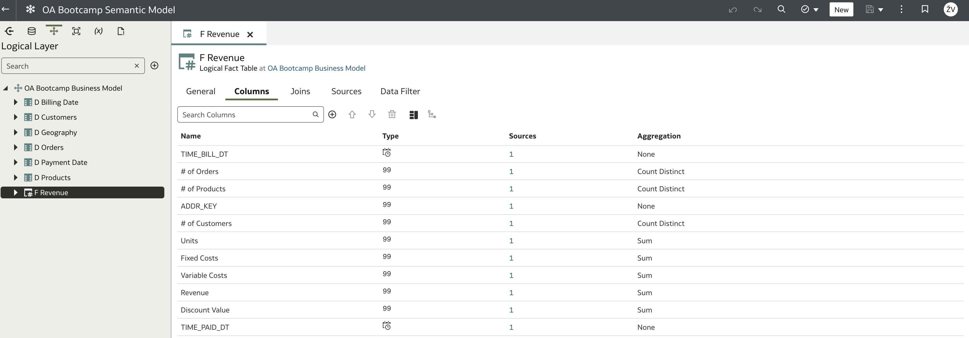
Simple Measure Calculations

Reviewing the existing measures, we often identify the need for additional business metrics that are not directly available in the source data. For example, let's create the following measures:

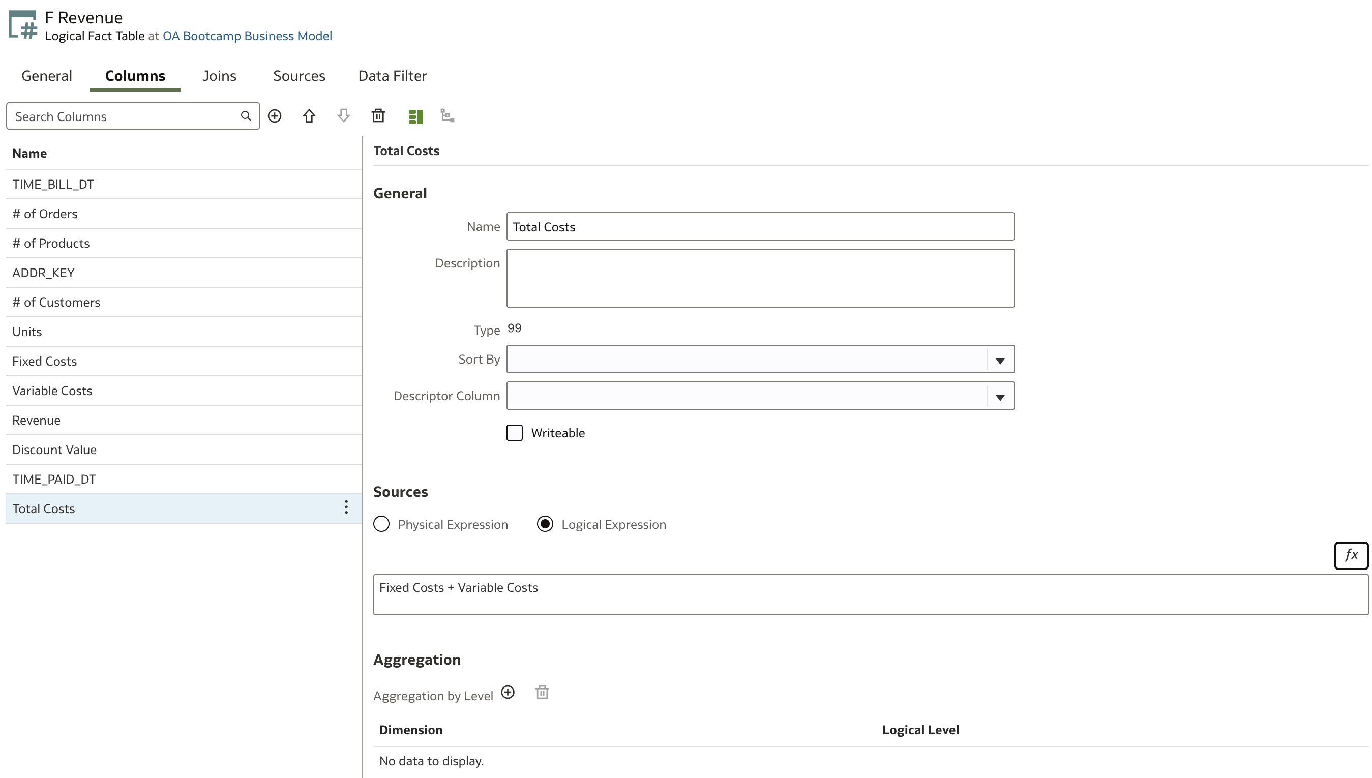
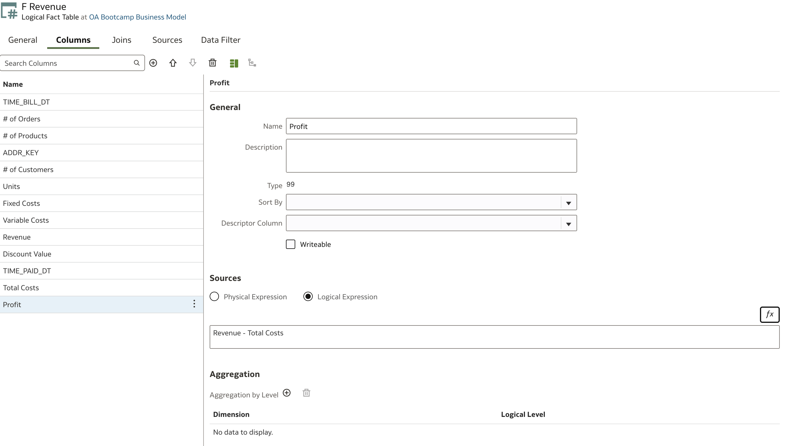
• Total Costs = Fixed Costs + Variable Costs
• Profit = Revenue - Total Costs
• Profit Margin % = Profit / Revenue * 100

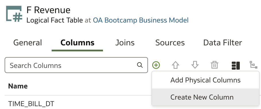
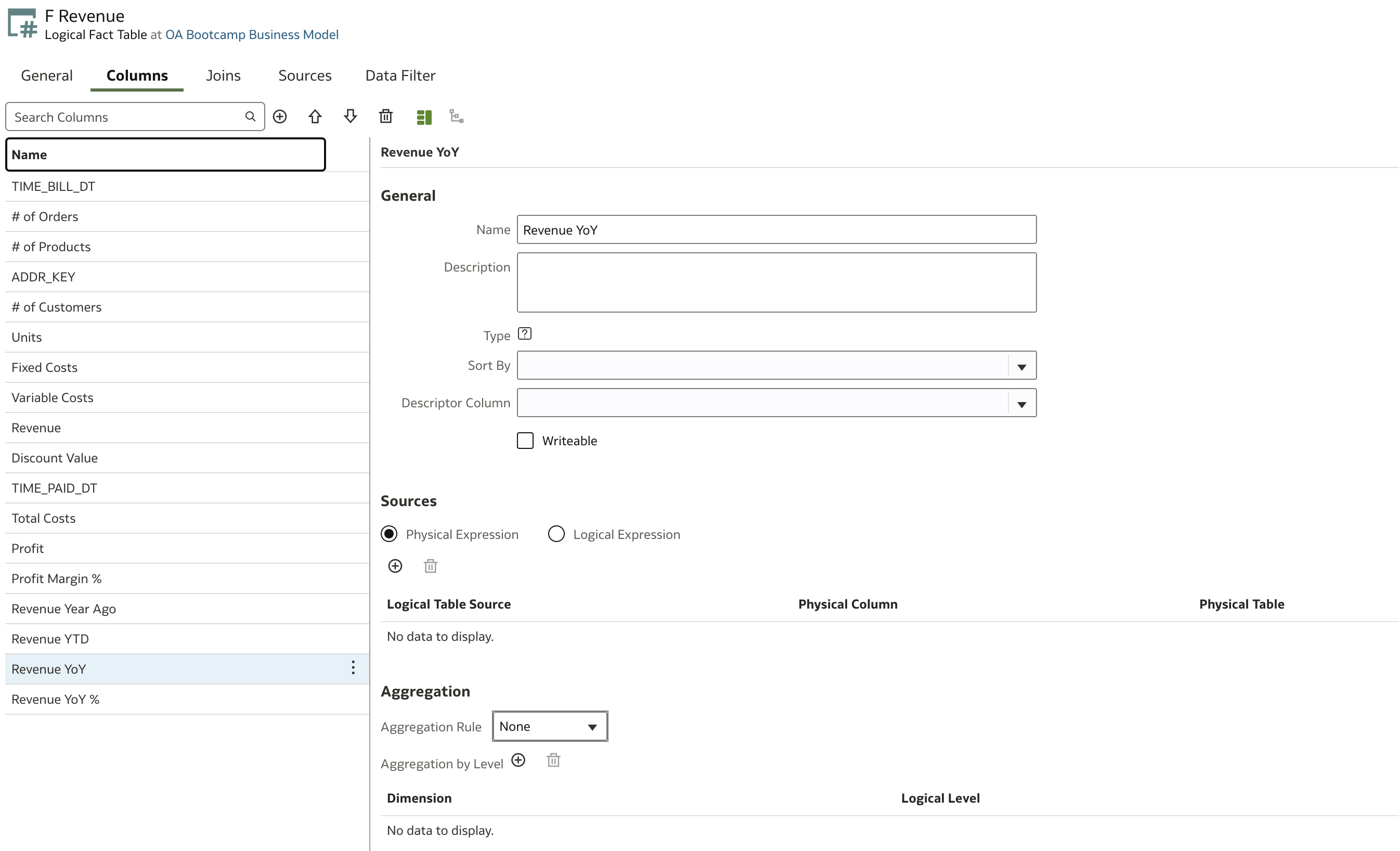
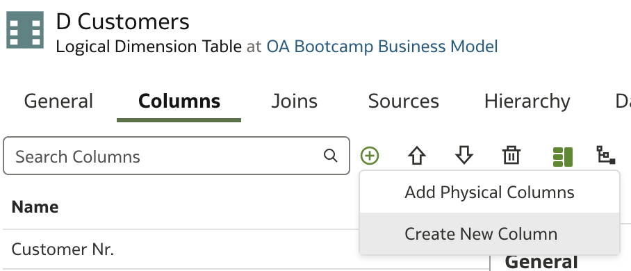
To add a new measure, start by clicking on the plus icon next to Search Columns and select Create New Column.

This action adds a new row for your column in the Columns list.

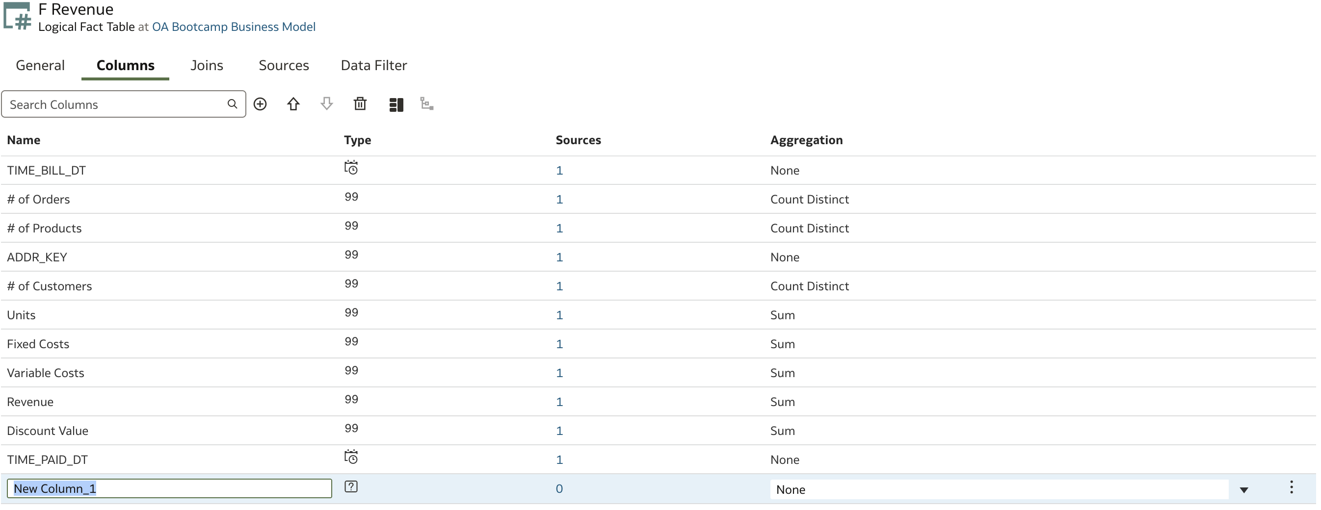
Click on the Details Icon (located above the list):

Name your new column and then click Logical Expression in the Sources section.

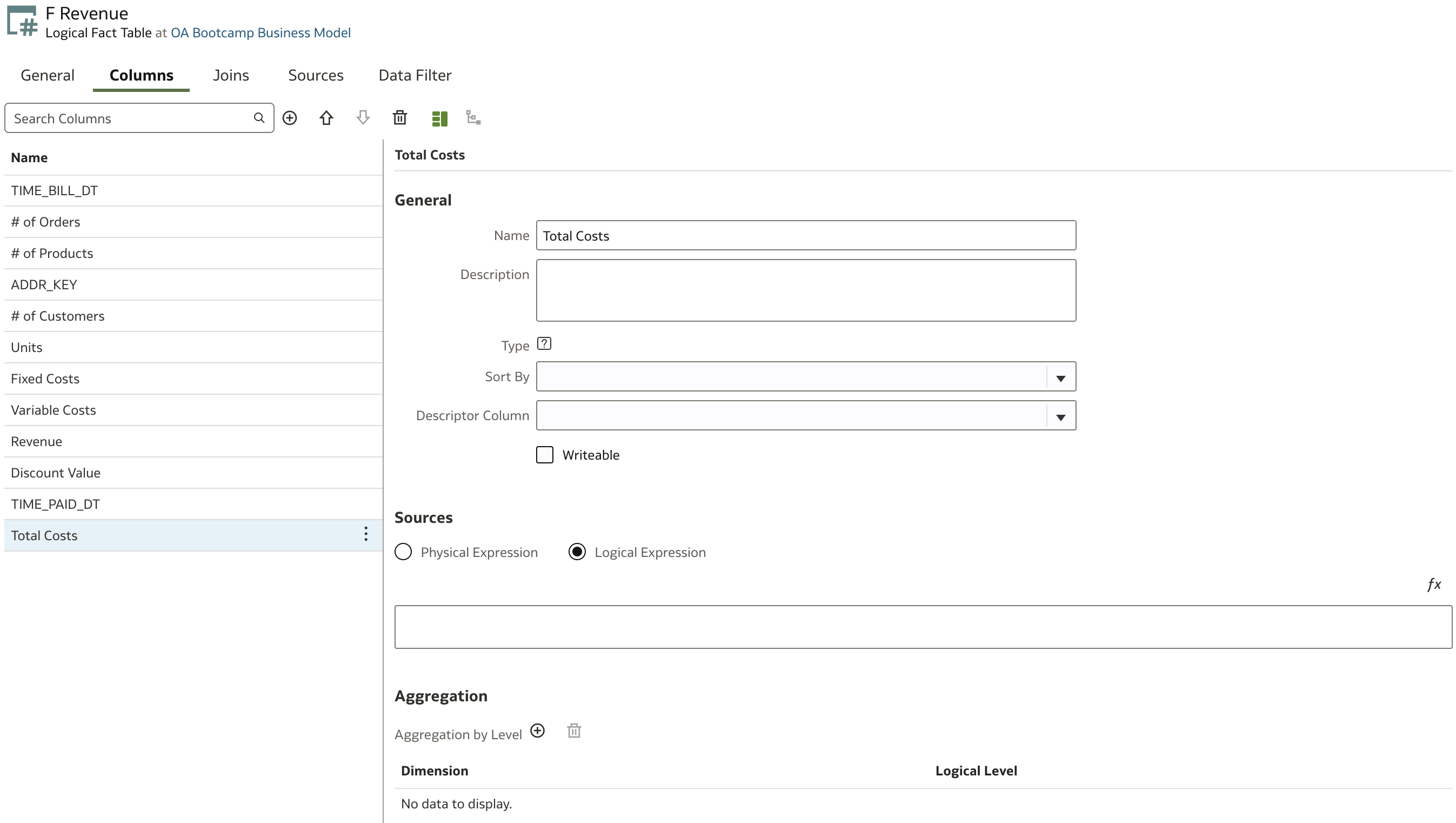
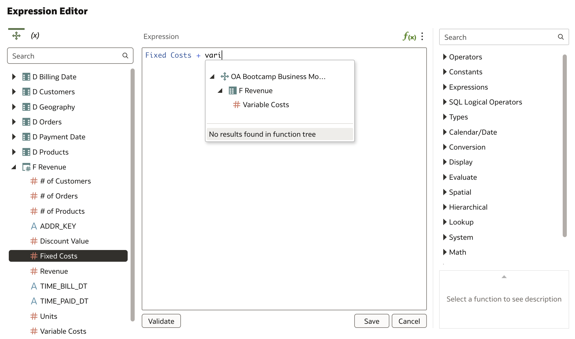
Simple formulas can be entered directly into the field in the Sources section. However, it is recommended to click the to open the Expression Editor. The Expression Editor not only provides syntax highlighting and function lookup, but also helps you validate and troubleshoot your formulas before saving them to the Business Model. This is especially useful for new users or for more complex logic.

Once your formula is validated, you can save it and proceed to create additional calculations as needed.

We can now create additional two calculations (Save your model first!):

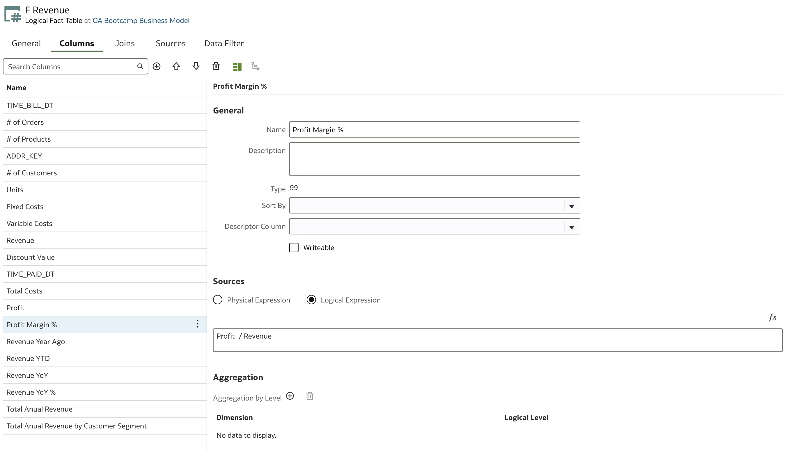
Note: Whether multiplying by 100 is required depends on your reporting needs; many data visualization tools allow you to format values as percentages, automatically multiplying by 100 for display purposes.

We have now created three measures which are available to all users—so there is no need for users to create these measures individually in their reports. This centralizes business logic and ensures consistency.

Next, let's look at a special type of calculation frequently used in business analytics: Time Series Calculations.

Time Series Calculations

Time Series Calculations enable users to perform powerful period-based comparisons, such as Year-over-Year (YoY), Month-to-Date (MTD), Year-to-Date (YTD), and rolling period averages. These calculations are built using specialized time-series functions within the semantic model and depend on a properly defined Time Dimension.

Why Chronological Keys Matter:
For Time Series Calculations to work correctly, your Time Dimension must have Chronological Keys defined. These keys ensure that Oracle Analytics understands the order of your time periods, allowing functions like AGO and TODATE to return accurate results. Without chronological keys, period-based calculations may produce incorrect or unpredictable outputs.

Common Time Series functions in Oracle Analytics include:

• AGO(): Returns the value of a measure from a previous time period (for example, Revenue from the prior year).
  Example: AGO("Revenue", "Year", 1) returns last year's revenue.
• TODATE(): Accumulates values from the beginning of a period to the current point (e.g., MTD, YTD).
  Example: TODATE("Revenue", "Year") returns year-to-date revenue.
• PERIODROLLING(): Returns a rolling sum (or other aggregate) over a defined period window.
  Example: PERIODROLLING("Revenue", 1, 3) returns the sum of revenue for the current and previous two periods.

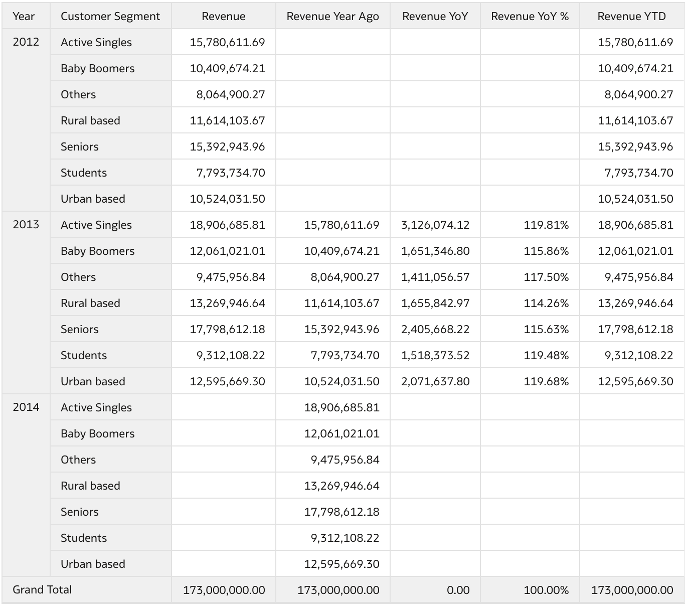
Let’s create two measures using AGO() and TODATE() for the measure Revenue. We’ll use D Billing Date as the Time Dimension.

Start by creating a new column as described earlier.

In the Expression Editor, if you are unsure about the function syntax, you can look it up on the right side of the editor. This is especially helpful for new users, as the editor provides function definitions and usage examples.

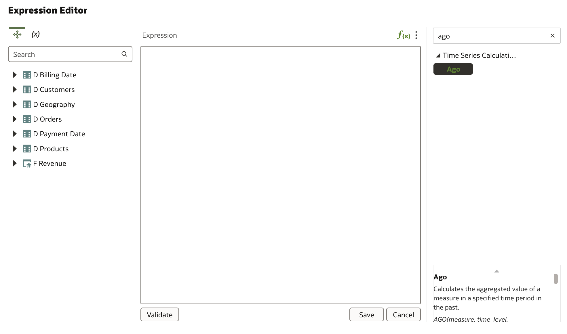
You can review detailed syntax and examples for any selected function. Double-clicking a function from the list copies its syntax into the Expression area, helping you get started quickly.

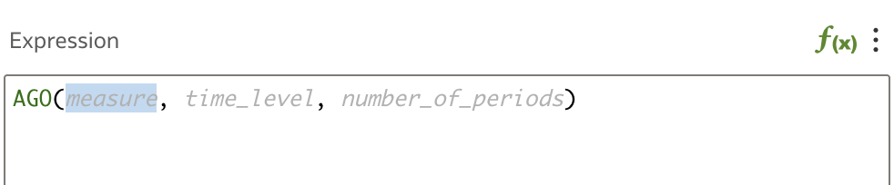
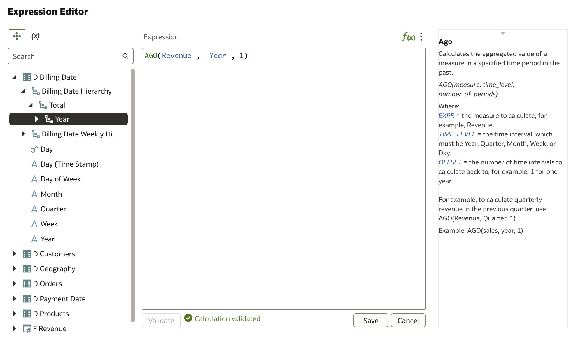
Enter the required attributes for your formula by referencing the business model and its tables/columns. Pay special attention to the TIME_LEVEL parameter, which is derived from the time hierarchy in your Time Dimension.

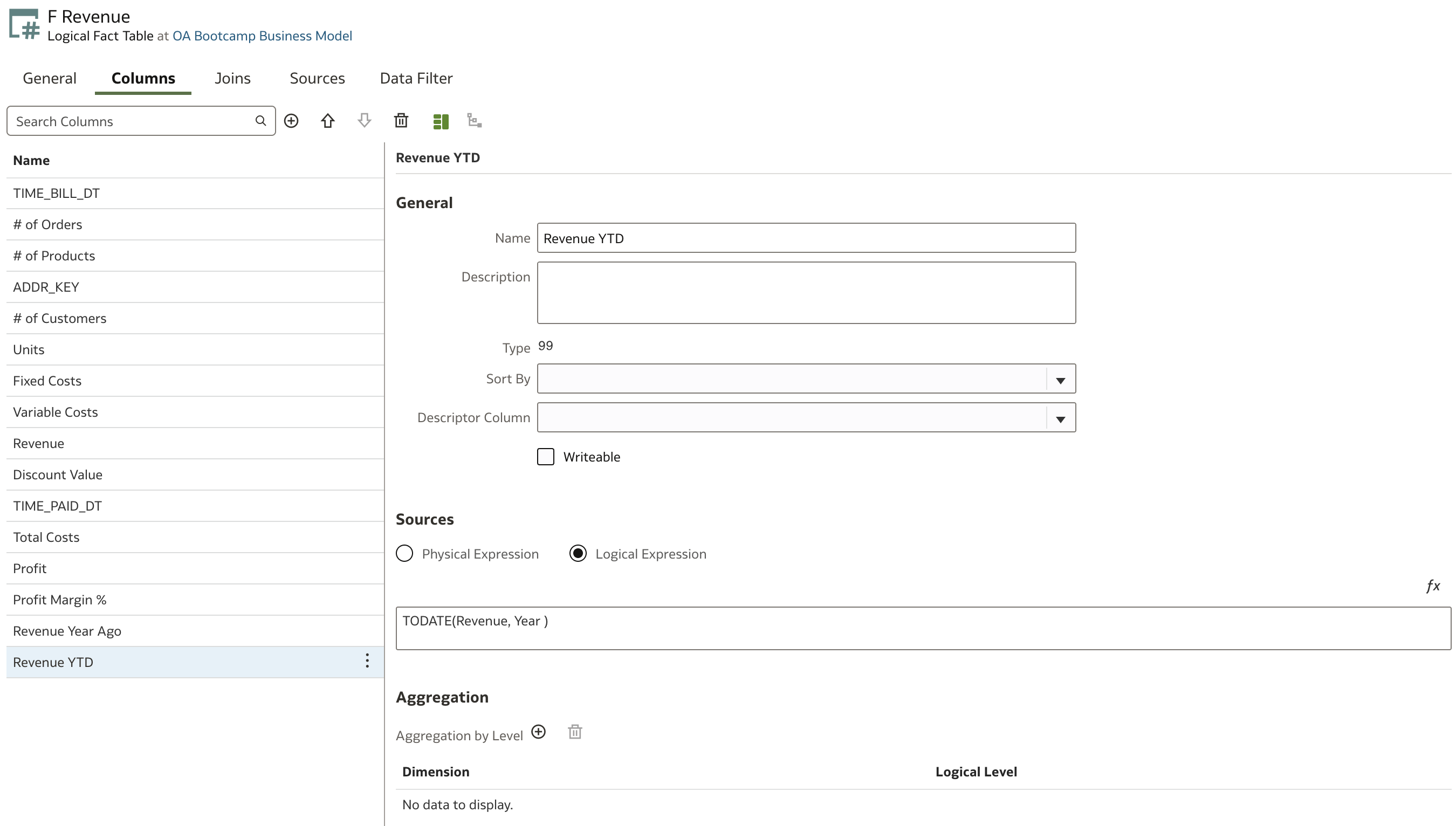
In a similar way, create a new time series measure: Revenue Year-to-Date using the TODATE() function.

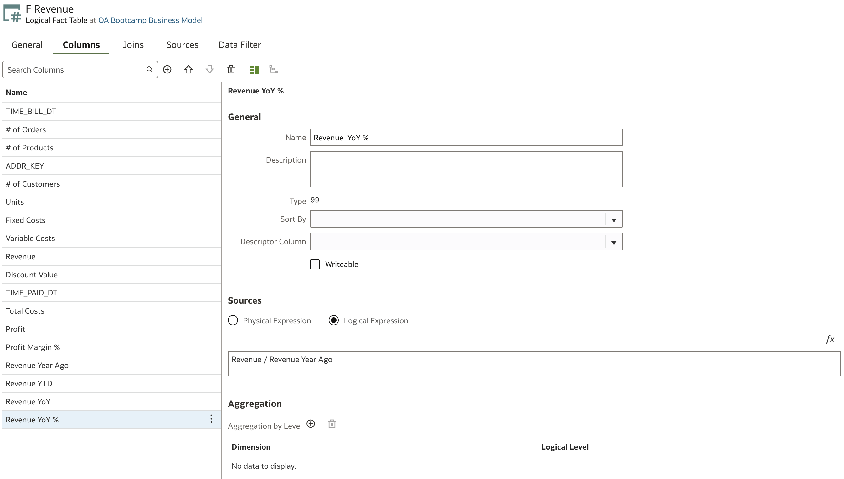
You can also create Revenue Year-over-Year and Revenue Year-over-Year Growth Index using combinations of these functions. For example, YoY Growth Index can be calculated as:
("Revenue" / AGO("Revenue", "Year", 1)) * 100

Level-Based Measures

Level-Based Measures are a powerful feature in the Business Model (Logical Layer) that allow developers to create aggregated measures at a specific dimension level. Regardless of how the data is grouped in an analysis, these measures always present data at the required aggregation level.

A Level-Based Measure is a metric (such as Revenue or Sales) that is pre-aggregated at a specific hierarchy level—such as Year, Region, or Product Brand—instead of dynamically responding to the query level.

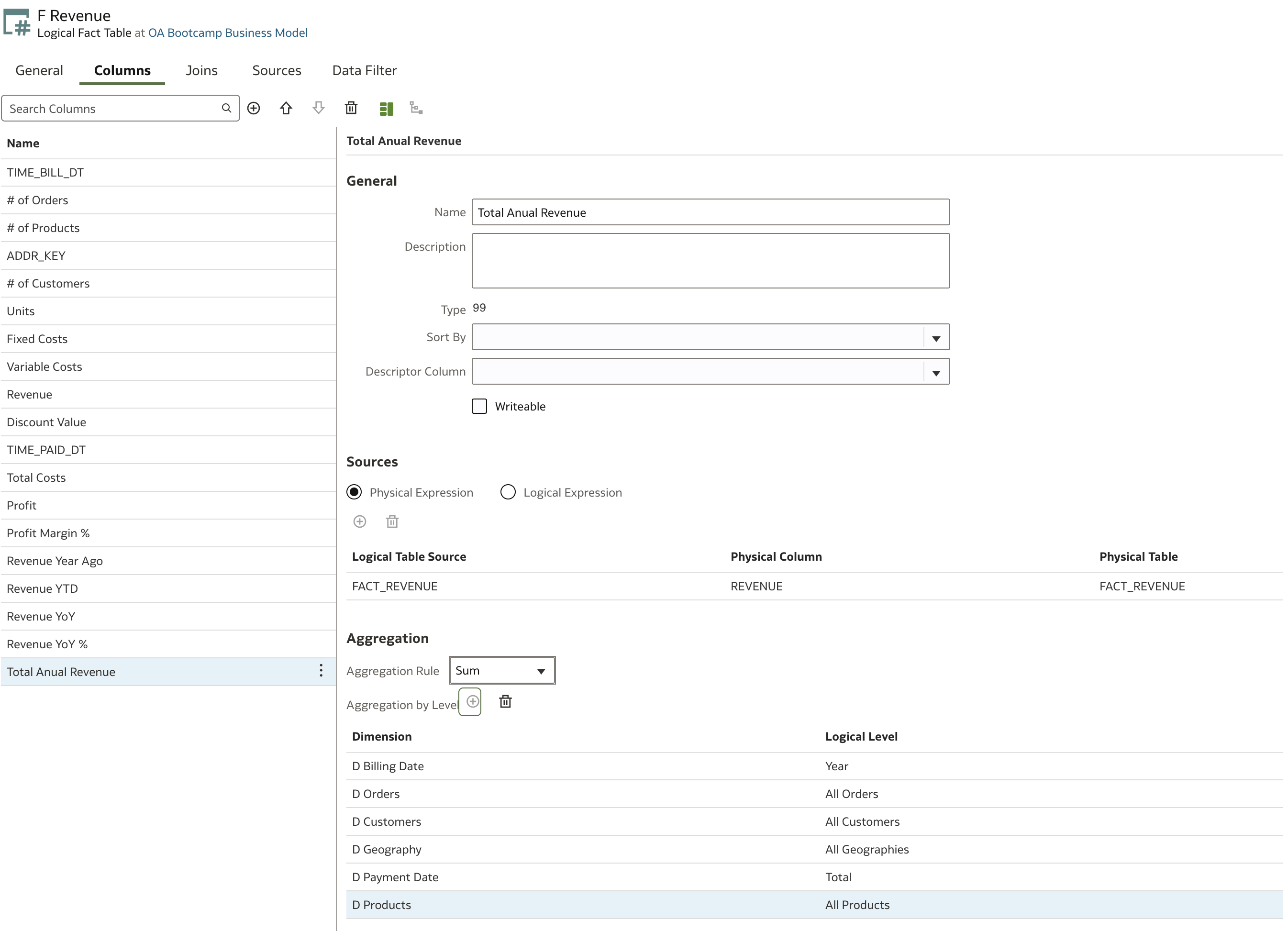
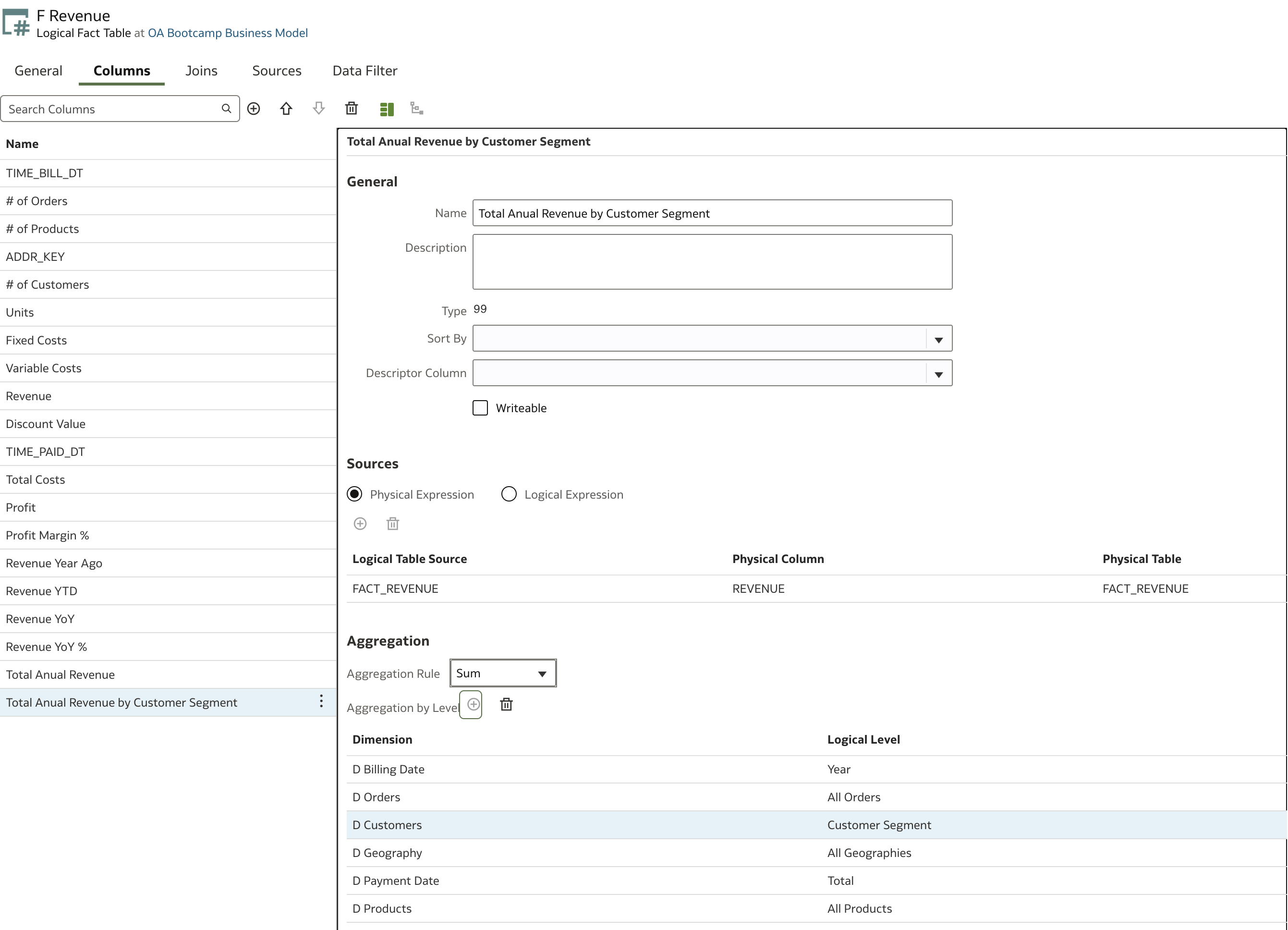
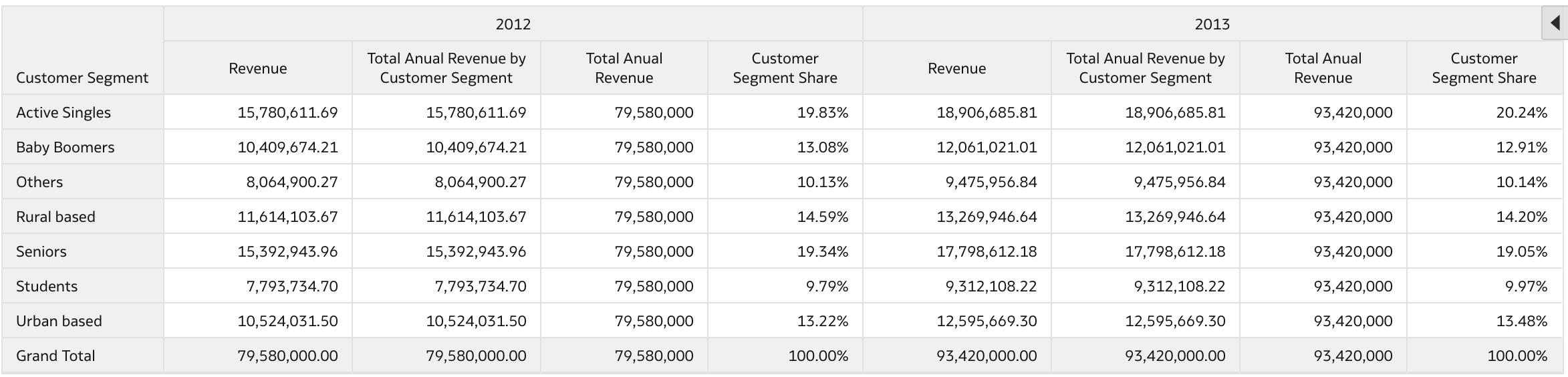
Let’s create a Total Annual Revenue measure as an example. From its name, we know that we need to aggregate all revenues by all dimensions at their top level, except for Year.

Here, we use a Physical Expression rather than a Logical Expression as in previous cases. First, specify the base measure for your level-based measure (in this case, Revenue).

Then, set up the aggregation:

• Select an Aggregation Rule (SUM in this example)
• Define levels for all dimensions: set all Logical Levels to the top level except for the D Billing Date dimension, where you set Logical Level to Year.

Why set all other dimensions to the top level?
By setting all other dimensions to their top levels, you ensure that your measure aggregates across the entire dataset except for the dimension of interest (e.g., Year). This is crucial for calculations like market share, ratios, or benchmarks, where you often need a total value to use as a denominator or reference.

This approach is useful, for example, when calculating revenue shares by customer segments: you need the total revenue for a specific year to use as the denominator in the revenue share calculation by segments.

Now, let's add another level-based measure similar to the one above, except it aggregates on the D Customer dimension at the Customer Segment level.

Instead of creating a new measure from scratch, you can simply duplicate the existing column:

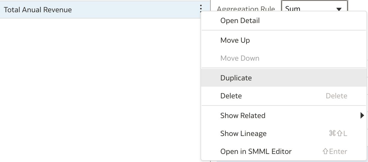
Now, update only the attributes that need to change:

Expressions in Dimension Tables

We can also create calculations or expressions on columns in Dimension Tables. This is helpful for enriching your data model with derived attributes that provide more business value.

For example, the D Customer logical table contains a column Birth Date:

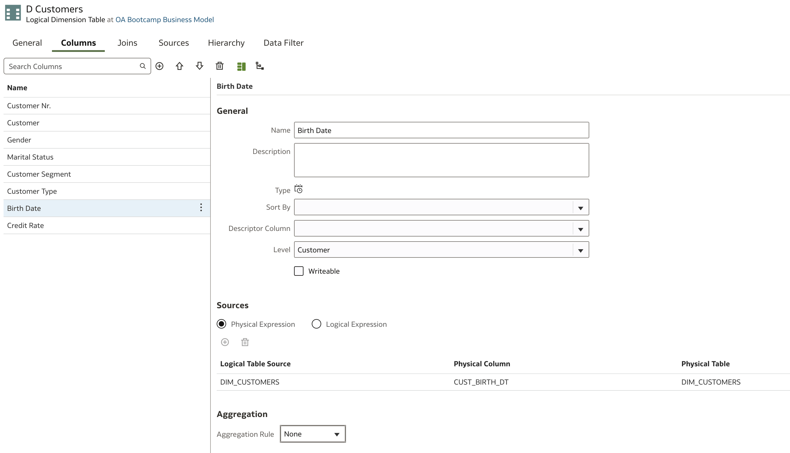
Instead of using birth date directly, it’s often more useful to have the customer’s age in years. We can introduce a new column Age that calculates the actual customer’s age based on the difference between CURRENT_DATE (a predefined session variable) and Birth Date.

First, create a new column in D Customer.

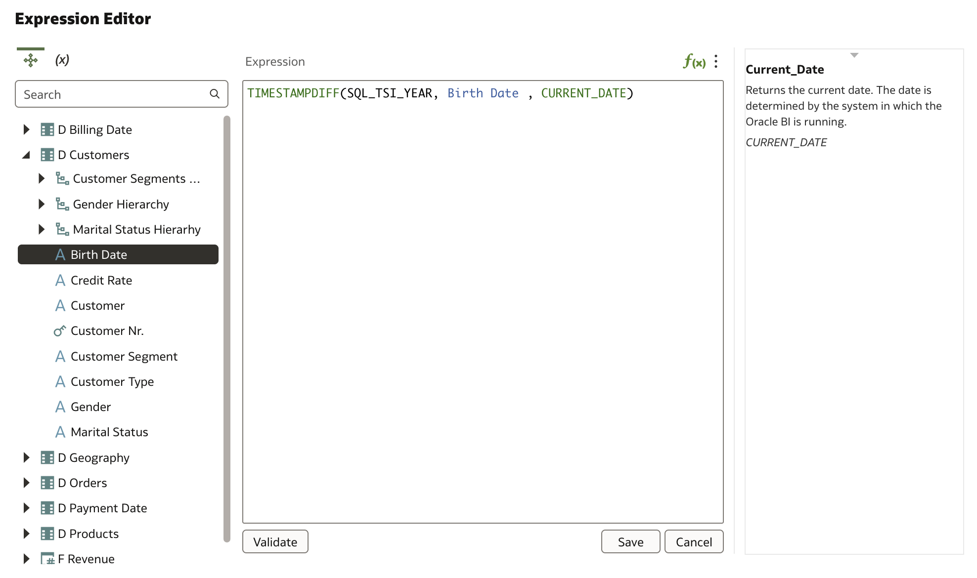
Using the Expression Editor, use the TimeStampDiff function to calculate the difference between CURRENT_DATE and Birth Date to derive Age.
Example:
TimeStampDiff(SQL_TSI_YEAR, "D Customer"."Birth Date", CURRENT_DATE)

Similarly, you can create additional derived columns in Dimension Tables as needed. This simple example shows that you are not limited to creating calculations only in fact tables; you can also use expressions within dimensions to enhance your data model.

Updating Subject Area

After adding new measures and calculations, these changes are not immediately reflected in your deployed Subject Area. To make them available to end-users, you need to update the Presentation Layer and deploy the changes to the BI Server.

Open the Presentation Layer first.

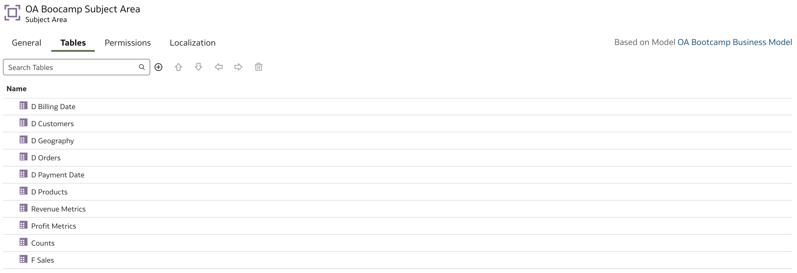
The Subject Area OA Bootcamp Subject Area currently looks like this:

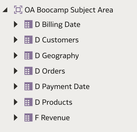
Since we have introduced several new measures, it’s a good opportunity to reorganize the presentation folder F Revenue for better user experience and easier maintenance. When you open the F Revenue presentation table, you might see all columns—even those not needed by end-users—and notice some are missing.

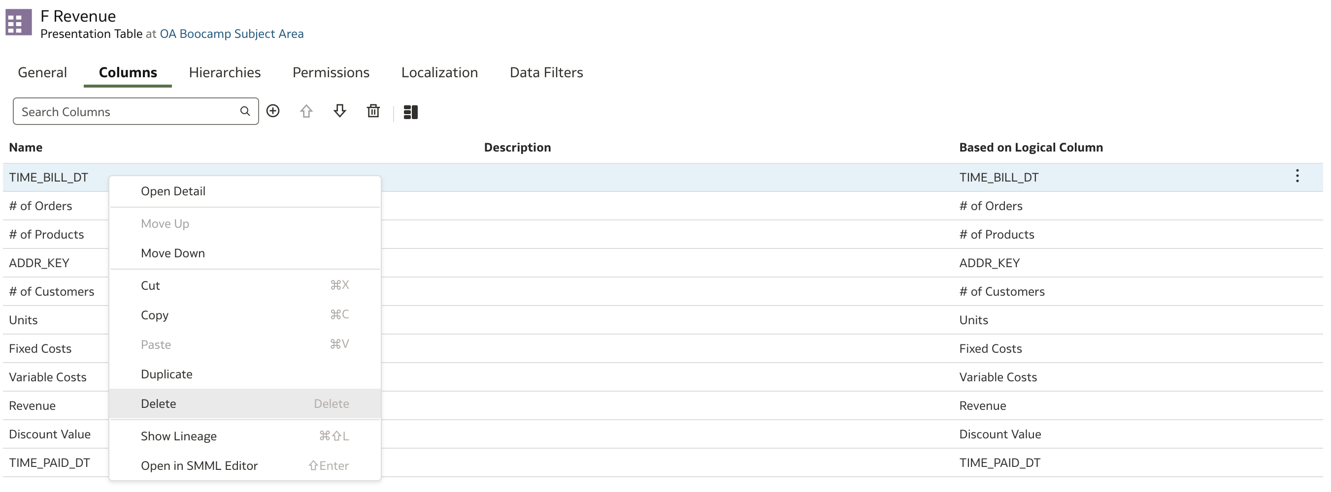
Start by deleting columns that are not required. These columns are:

• TIME_BILL_DT
• TIME_PAID_DT
• ADDR_KEY

Remove them to streamline your presentation table.

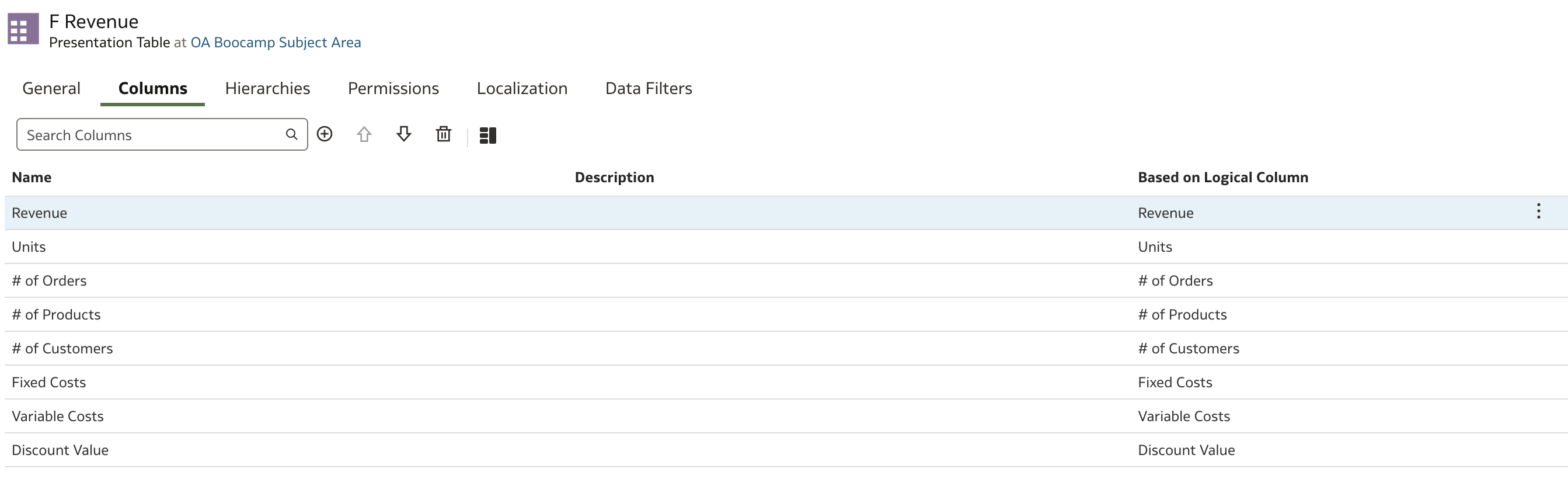
After deletion, the F Revenue presentation table looks like this:

Now, let’s further reorganize F Revenue by splitting measures into separate presentation tables based on their type: revenue-related, profit-related, and counts. This reorganization improves user navigation and makes it easier to find relevant metrics.

Create the following presentation tables:

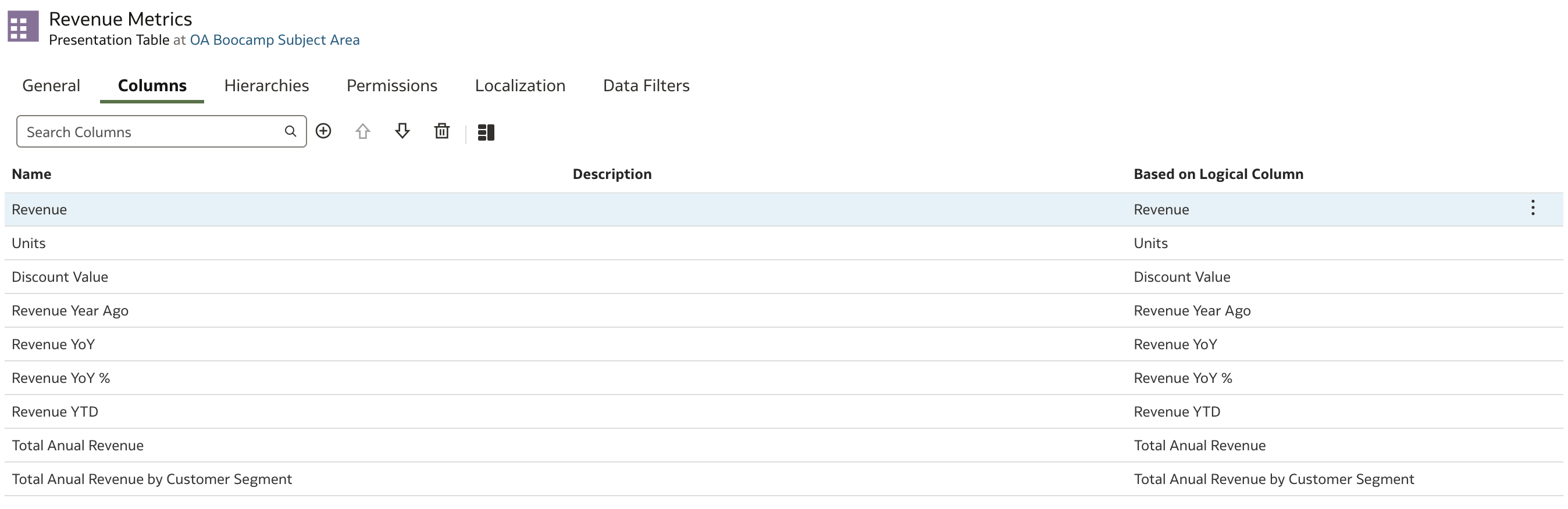
• Revenue Metrics
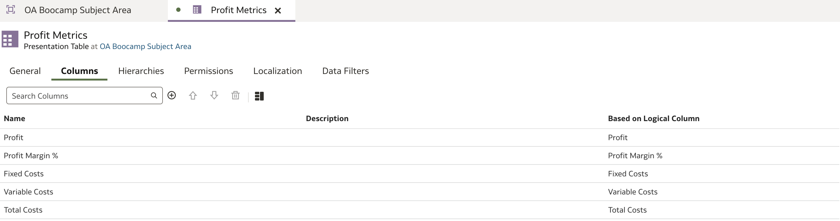
• Profit Metrics
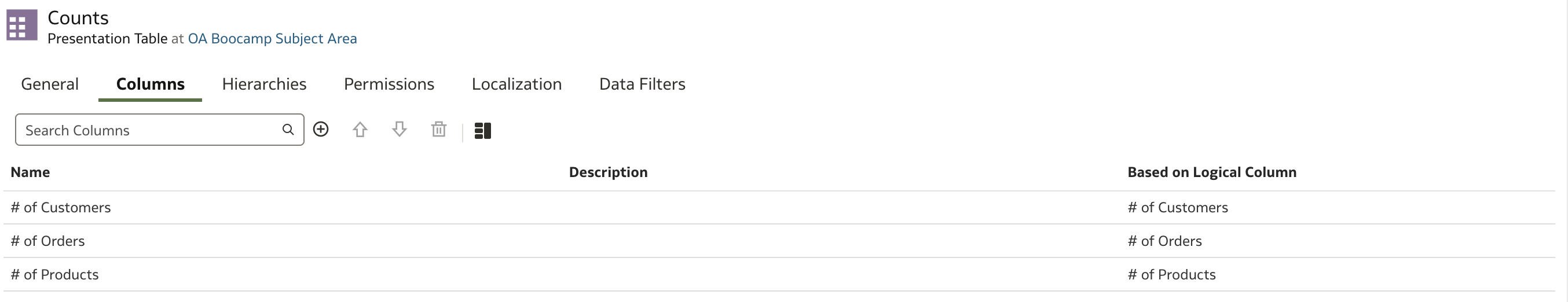
• Counts

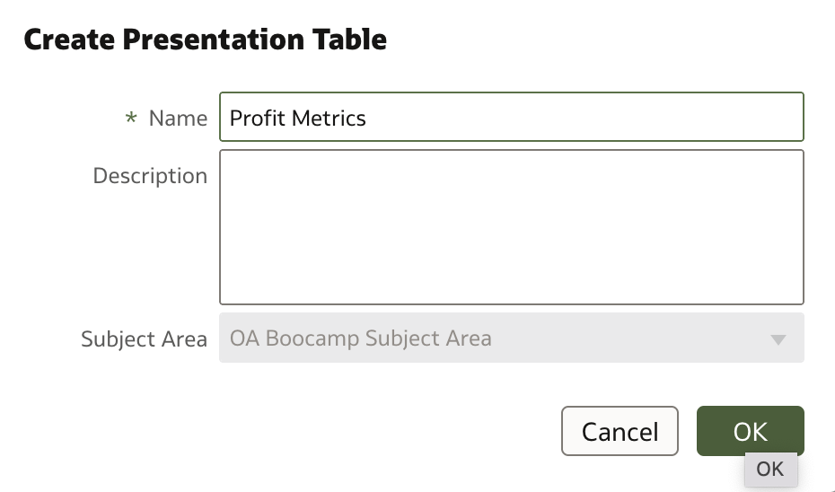
Open the Subject Area page and navigate to the Tables tab. Click on the plus icon to create a new Presentation Table.

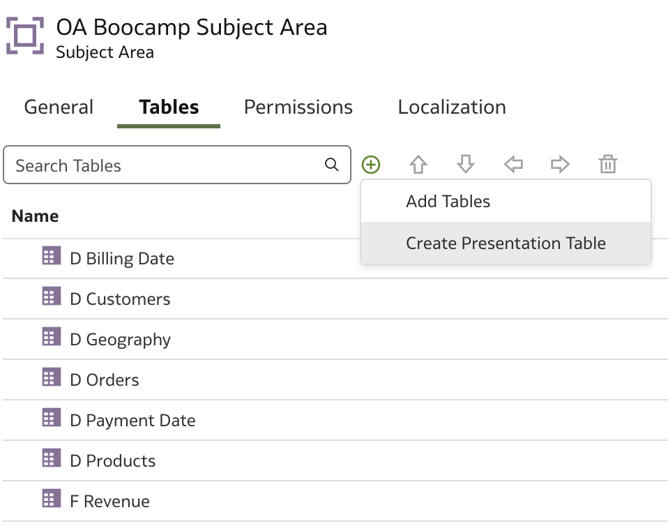
Enter the presentation table name Profit Metrics from the list above and click OK. Repeat this process for Counts as well.

Rename F Revenue to Revenue Metrics.

Open Profit Metrics. Add all profit-related columns into this presentation table. To do this, navigate to the Logical Layer in the navigation pane on the left, select all profit-related columns, and drag them onto the Columns area of the Profit Metrics presentation table page.

Repeat this process to add all # of ... columns into the Counts presentation table.

Open Revenue Metrics. Remove columns that have already been added to Profit Metrics or Counts, and then add any additional revenue-related metrics from the logical layer.

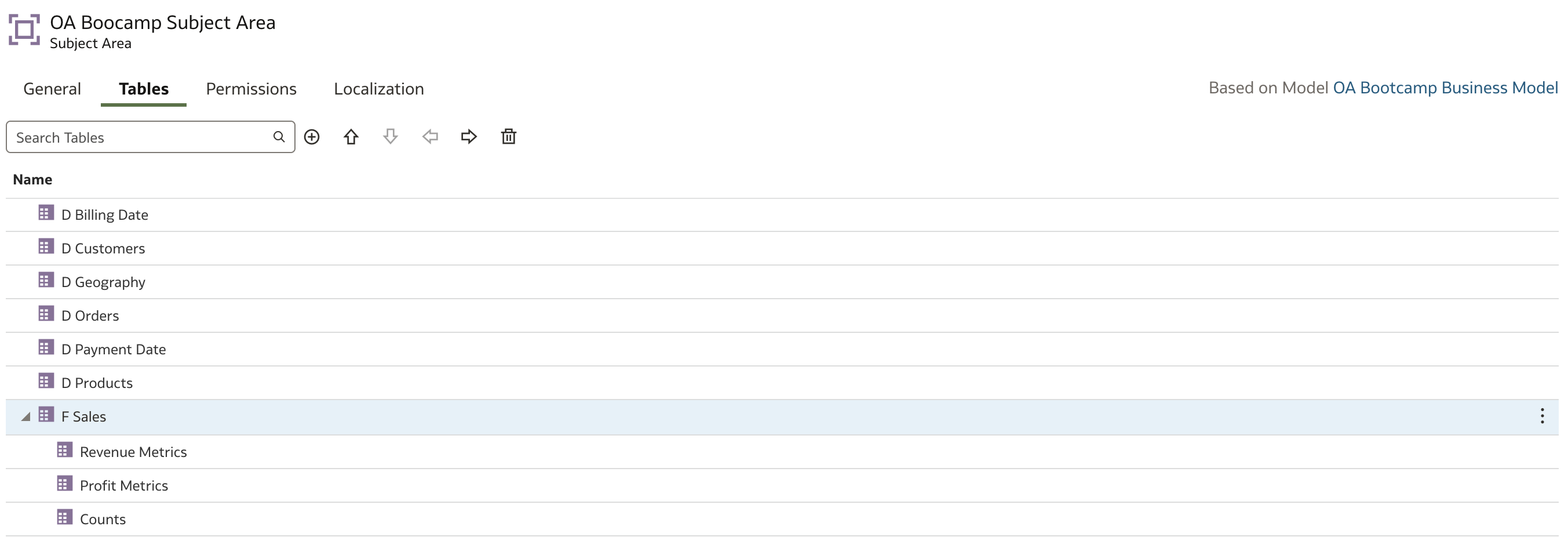
We have now created three presentation tables in our Subject Area. To keep the Subject Area organized and user-friendly, we’ll group these three presentation tables under a parent folder called F Sales. This reorganization improves user experience by making it easier for users to find related metrics and helps maintain the model as it grows.

First, create another new Presentation Table called F Sales.

Now, drag and drop all three previously created presentation tables (Revenue Metrics, Profit Metrics, and Counts) onto the F Sales presentation table.

You can now save your model, run a consistency check, and deploy it.

For added assurance, run the Advanced Consistency Check.

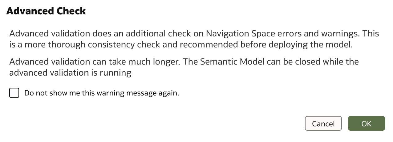
You’ll see a message indicating that the Advanced Consistency Check is running at the bottom-right of the screen:

Once the check completes (successfully or not), the result is displayed at the bottom-right. If successful, proceed to deploy the model.

Review and Test Changes

After deploying, the first test is to verify that your presentation tables are properly configured and displayed. You should now see a single folder F Sales with the following subfolders/presentation tables:

• Revenue Metrics
• Profit Metrics
• Counts

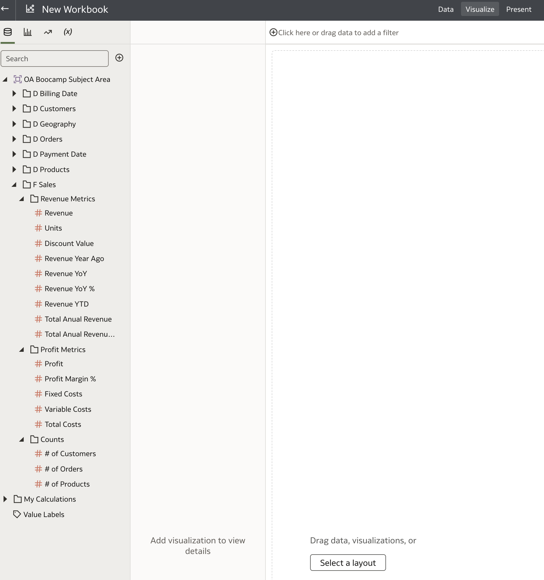
More importantly, test the new metrics to ensure they return correct results.

Start by checking simple calculations:

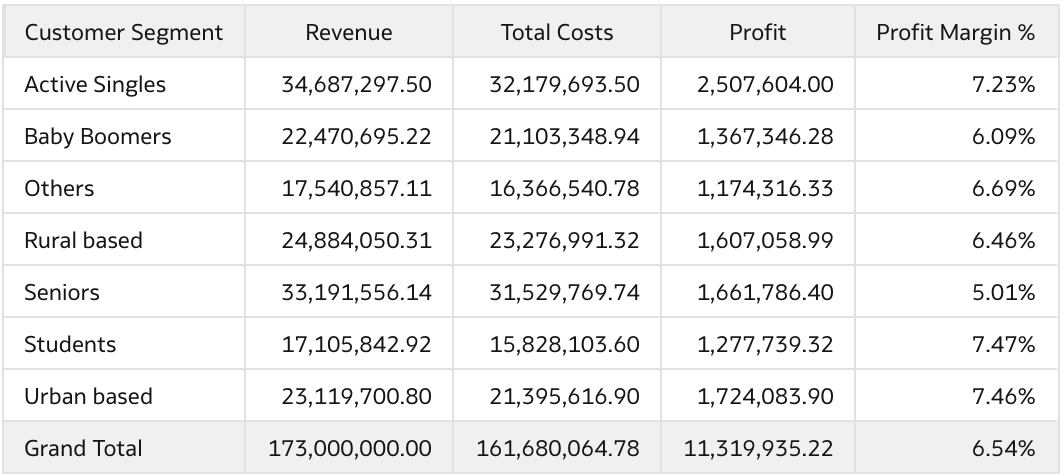
You should see all measures (Total Costs, Profit, and Profit Margin %) calculated properly.

Next, check Time Series calculations:

Lastly, verify the newly introduced Level-Based Measures:

---

Summary

In this guide, we covered several key types of calculations in Oracle Analytics:

• Simple Measures: Direct formulas and business logic, such as profit and margin calculations.
• Time Series Calculations: Functions such as AGO and TODATE for period-based analysis (e.g., Year-over-Year, Year-to-Date).
• Level-Based Measures: Aggregations at specific dimension levels, enabling advanced analytics like market share and benchmarking.
• Expressions in Dimensions: Derived attributes within dimension tables, such as customer age.

Business Benefits:
Building calculations in the semantic model brings significant business benefits:

• Reusability: Define once, use everywhere—ensuring consistent logic across reports and dashboards.
• Performance Optimization: Centralized logic can be optimized for better query performance.
• Easier Maintenance: Updates and corrections are made in one place, reducing errors and effort.

Important:
Always thoroughly test and validate your calculations before deploying changes to production. This ensures accuracy, reliability, and a smooth experience for your business users.