Physical Layer
The Physical Layer is the foundational layer in the three-tier semantic modeling architecture. It plays a crucial role in connecting Oracle Analytics to external data sources—such as databases—and determines how raw data is retrieved and structured before being transformed into business-friendly formats in the subsequent Logical and Presentation Layers. By establishing the groundwork for data connectivity, structure, and relationships, the Physical Layer ensures that downstream modeling and analytics are both reliable and performant.
What Does the Physical Layer Include?
-
Connections to data sources (e.g., relational databases on-premises or in the cloud, such as Oracle Autonomous Database, Snowflake, SQL Server, etc.). Connections are defined system-wide and can be reused across different models. As we have already learned, they can be regular or system connections.
-
Schemas and tables/views: When building the Physical Layer, you can import tables (or, preferably, their definitions). In addition to tables, views or SQL expressions are also supported. Once imported, tables can be renamed without affecting the underlying database tables. It's best practice to create aliases for imported tables and work with these aliases rather than directly with database tables—a topic we will revisit later.
-
Joins between tables define relationships within the model. The BI Server generates queries executed against database tables using these join definitions. Therefore, join definitions are critical and must be handled with care. There is no requirement for a specific physical model in the database before import—it can be 3NF, star, snowflake, or even a flat, denormalized table. The Physical Layer imposes no constraints, whereas the Logical Layer will require a star schema.
-
Optional data source filters, caching settings, and descriptions:
- Data source filters can be directly applied to physical data sources, enabling row-level security.
- You can define caching strategies for each table in the Physical Layer.
Why Is the Physical Layer Important?
- It abstracts raw data from end users. Business users never have to deal with tables or SQL—they interact with the Logical and Presentation Layers.
- It enables performance tuning at the lowest level.
- It gives developers and administrators control over source metadata, joins, and security before data is transformed into business-friendly formats.
In this lab, we will walk through the process of creating a Physical Layer. Let’s get started!
Creating a New Database
First, navigate to the Physical Layer.
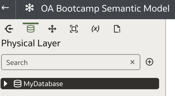
You may notice a default database called MyDatabase. This is a placeholder and needs updating. You can either update it or, as we recommend, start from scratch by deleting any existing database (be cautious with deletions unless you are working in a new semantic model!).
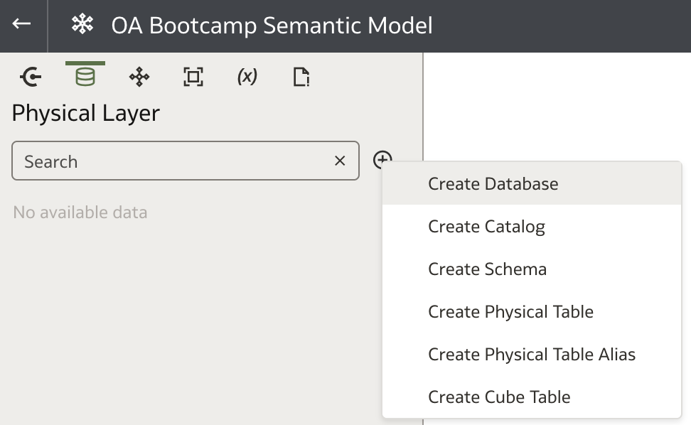
To create a new database, click the plus icon (![]() ) next to the Search field and select Create Database:
) next to the Search field and select Create Database:
The Create Database dialog will appear. Enter a Name, optionally a Description, and select your Database Type. In our case, choose Oracle Autonomous Data Warehouse.
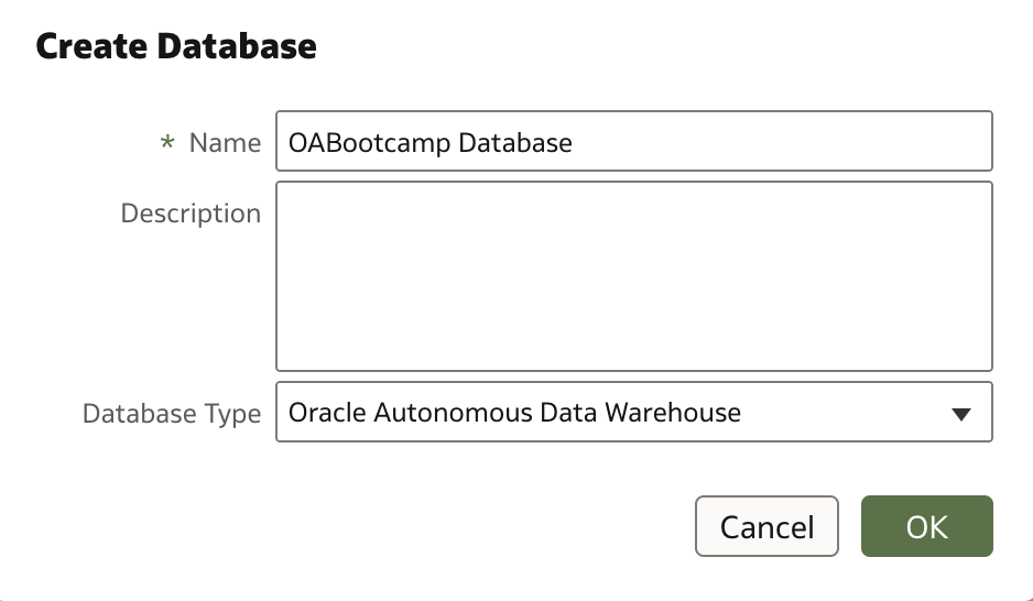
Click Ok to create the new database.
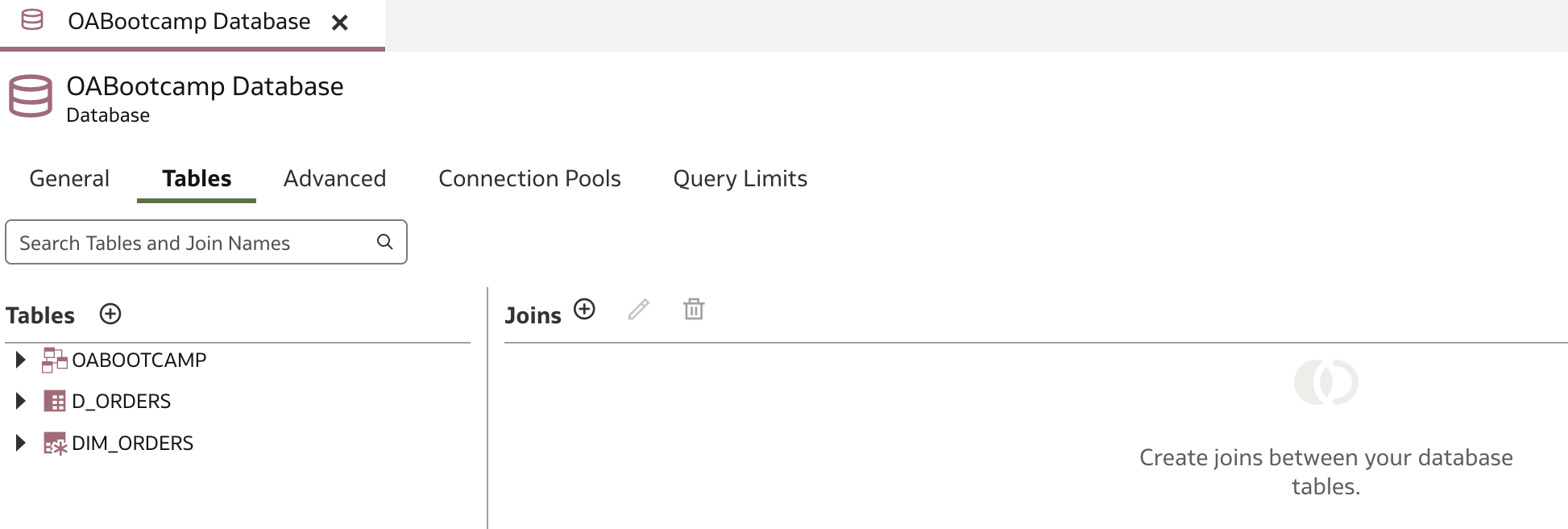
The newly created database will open in the main canvas area, currently empty:
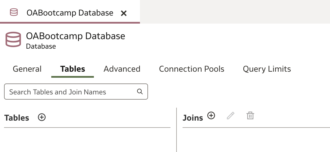
Your database is defined by five tabs:
- General: General database definitions like database name and type.
- Tables: Lists all physical tables (and aliases) in the database.
- Advanced: Configure database-specific SQL behavior.
- Connection Pools: Shows all connection pools defined for the database.
- Query Limits: Set query-level restrictions at the database level.
For this exercise, we will focus on Tables and Connection Pools.
Connection Pools
A connection pool defines how Oracle Analytics connects to the database—including credentials, maximum connections, timeouts, and more. You can define multiple connection pools for a database. For example, it's good practice to have a separate connection pool for variable initialization, so typically you might expect more than one connection pool here. For our lab, one will suffice.
Navigate to the Connection Pools tab. As expected, the list is empty.
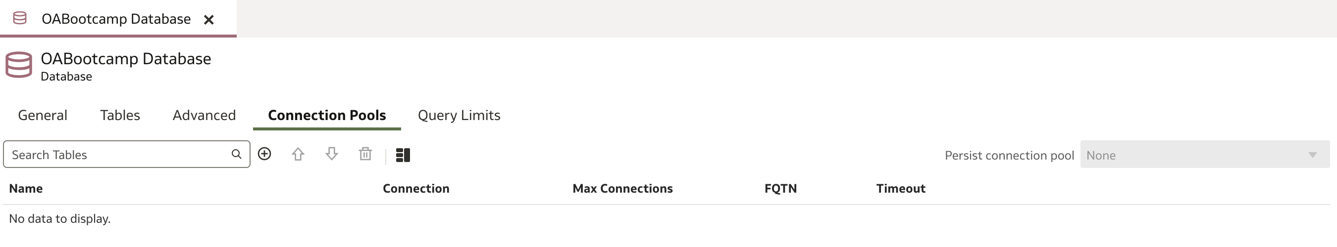
To enable database connectivity, you need to create at least one connection pool.
Click the plus icon (![]() ) next to the Search field. This will automatically add a new connection pool.
) next to the Search field. This will automatically add a new connection pool.
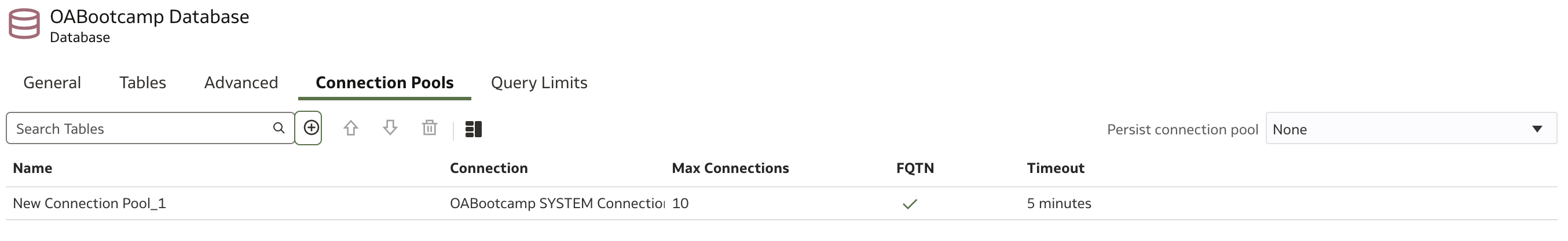
Click the details icon:
This icon behaves consistently throughout the Semantic Modeler: it opens the details for the selected object—in this case, the connection pool New Connection Pool_1.
You can now update the connection pool details, such as the Name. Let's rename it to OA Bootcamp Connection Pool - Main. We will explore connection pools in greater depth in later chapters.
Save your progress so far. The save icon (diskette) is located at the top right (![]() ).
).
Tables
The Tables section is the core of the database definition. Here, you import tables, views, or SQL query results, and define joins between tables.
We'll start by importing dimension tables. There are four dimension tables (tables beginning with D_). There are several ways to add tables, but we'll use the simplest: drag and drop.
In the navigation bar on the left, switch to the Connections tab. Expand Schemas and select the OABOOTCAMP schema. Click on the following tables:
- D_CUSTOMERS
- D_GEOGRAPHY
- D_PRODUCTS
- D_TIME
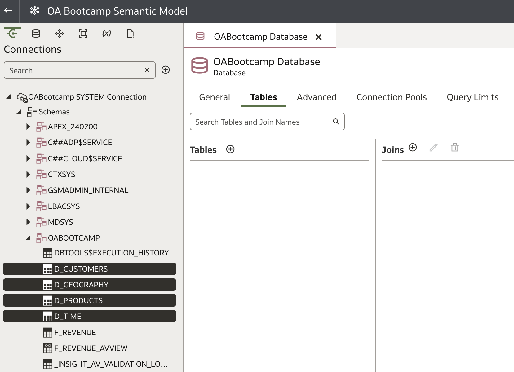
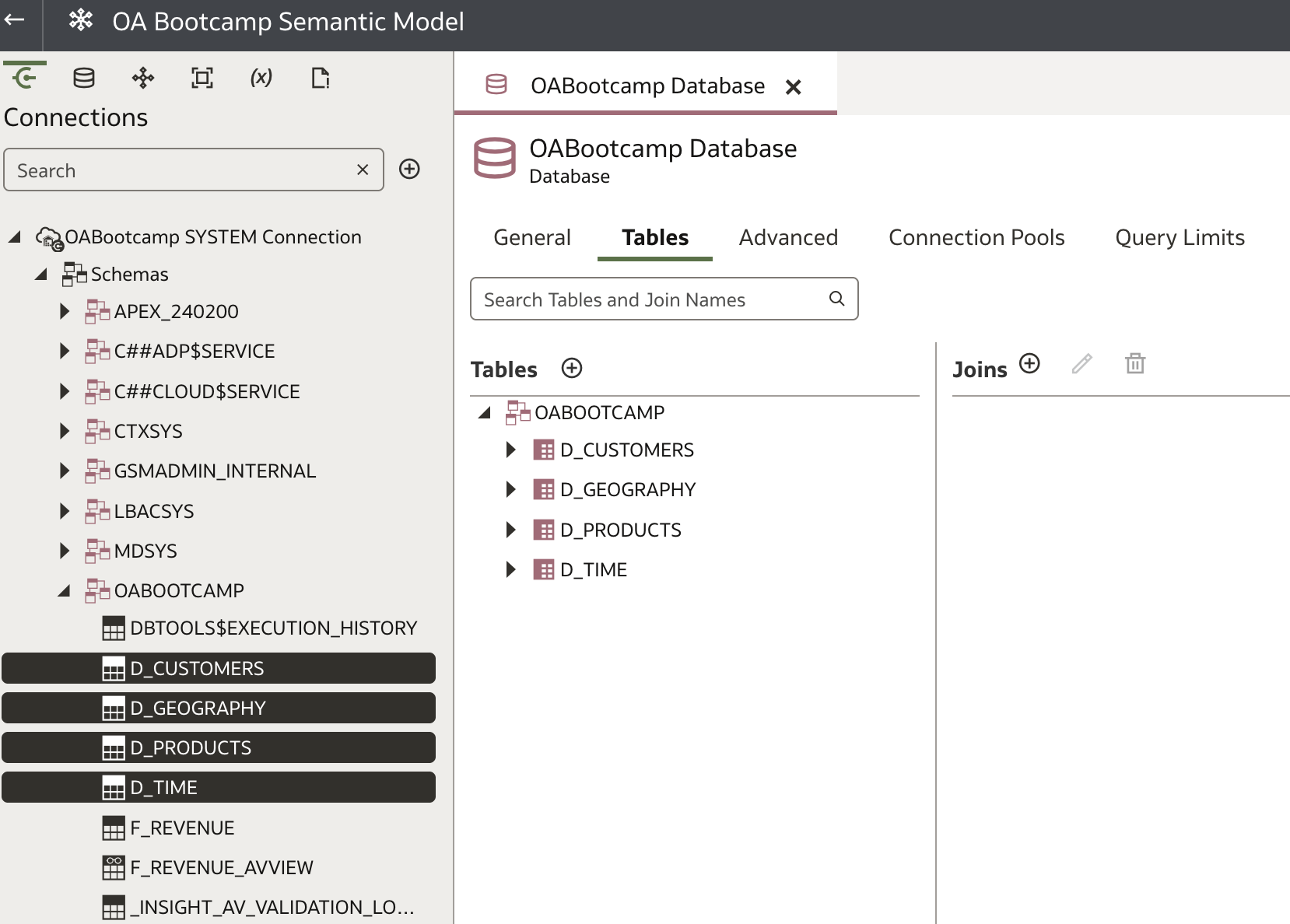
Drag the selected tables onto the Tables section of the canvas and drop them there. All four dimension tables should now appear in the database.
Alternatively, you can add a new table by clicking the plus sign (![]() ) next to Tables.
) next to Tables.
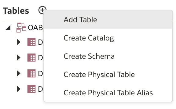
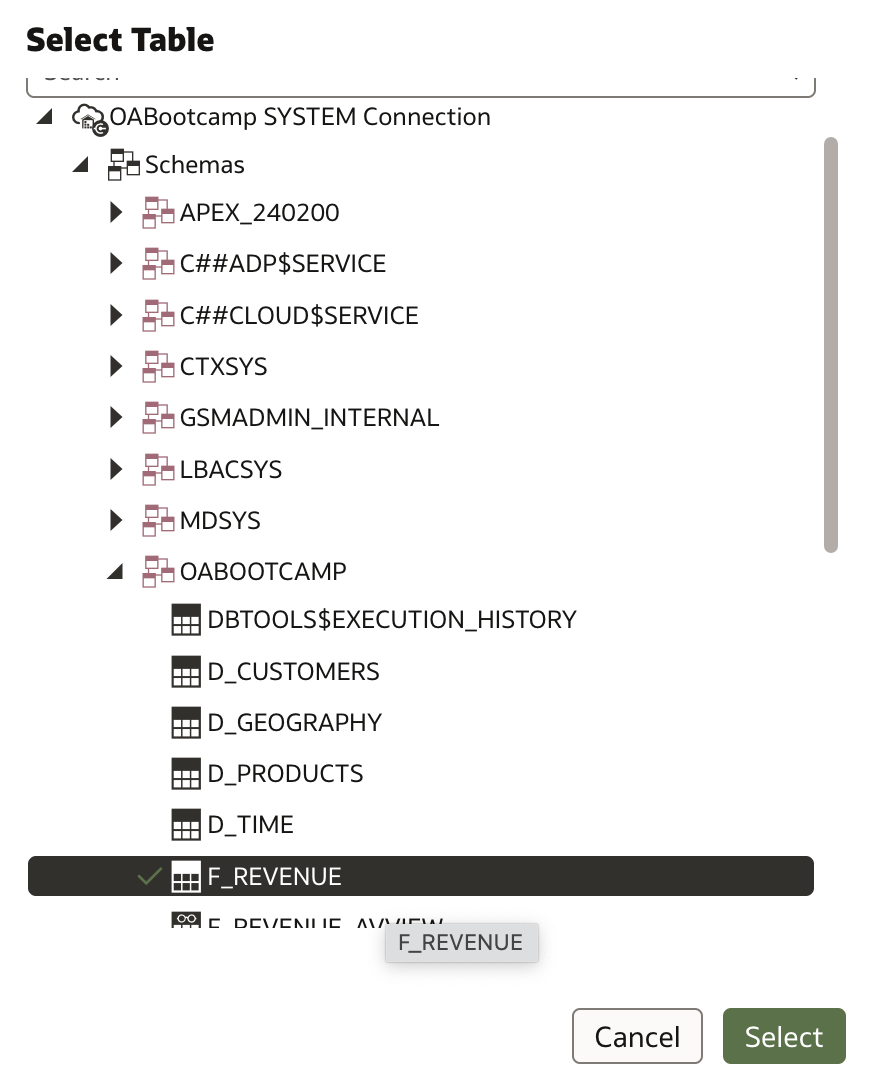
When clicked, a menu appears. Select Add Table. In the Select Table dialog, expand Schemas and navigate to the fact table F_REVENUE. Select it and click Select.
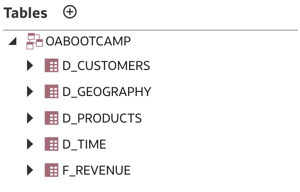
After refreshing, you should see five tables: four dimension tables and one fact table.
Let’s add one more table—a new dimension table called D_ORDERS, whose columns will be a subset of columns from the F_REVENUE table.
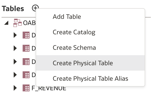
Click the plus sign (![]() ) next to Tables again.
) next to Tables again.
This time, select Create Physical Table.
In the first step of the Create Physical Table dialog, provide a name for the new table—D_ORDERS.
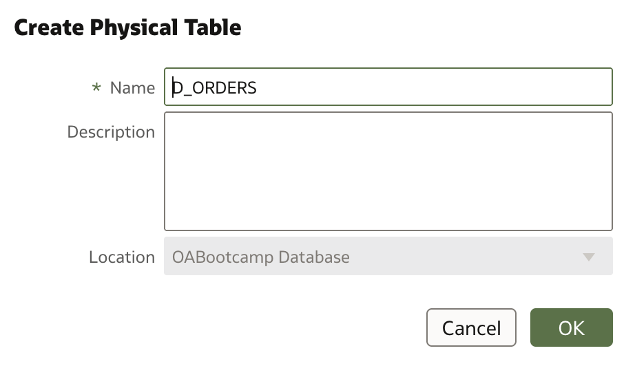
Click Ok to continue.
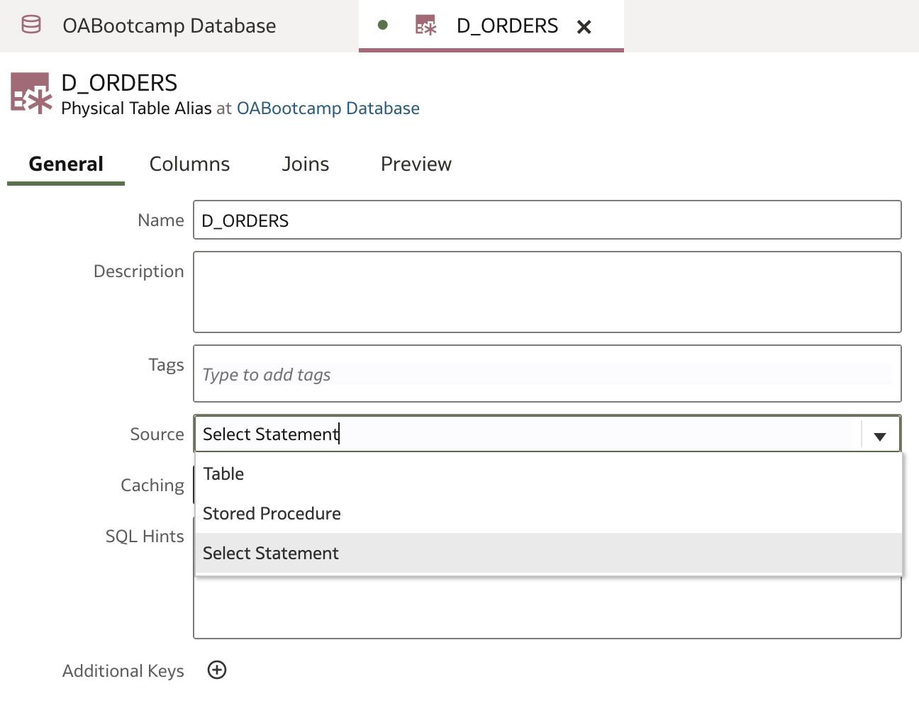
A new tab for D_ORDERS opens. There are several ways to define columns for this new Physical Table. We will use a SQL Query to populate the table.
First, navigate to the General tab. Observe that Source is set to Table. Change it to Select Statement.
Go to the Columns tab and enter the following SQL code in the Select Statement:
SELECT  ORDER_KEY,
        ORDER_STATUS,
        CHANNEL_NAME,
        TIME_BILL_DT,
        TIME_PAID_DT
FROM F_REVENUE
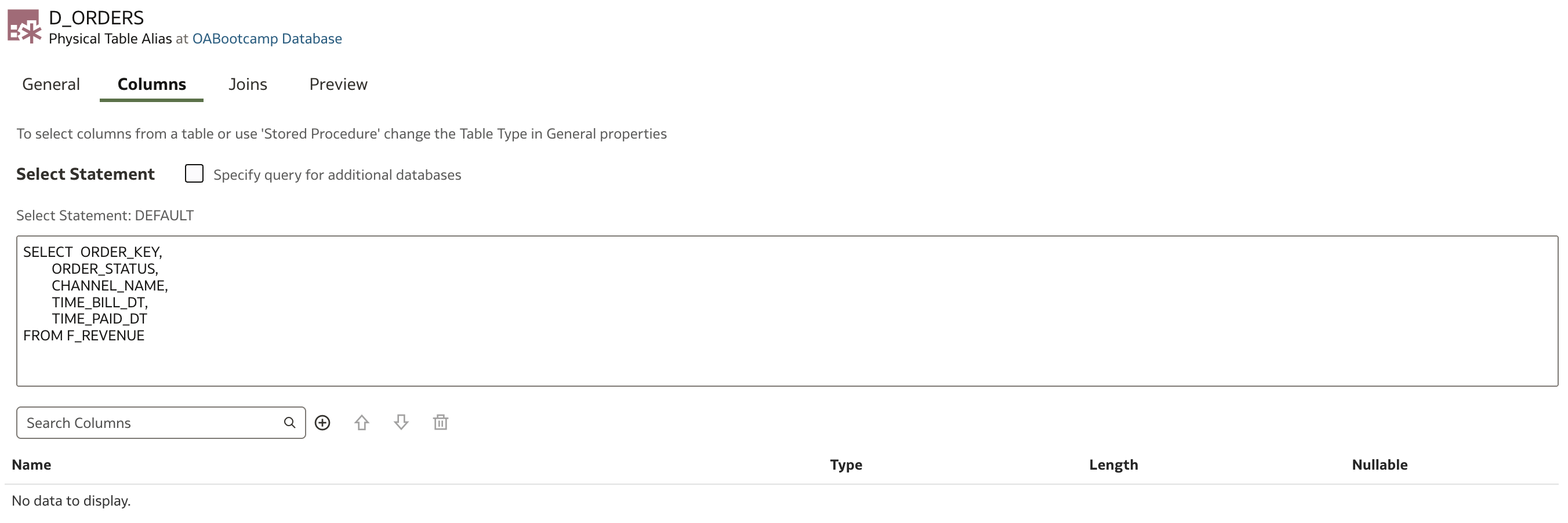
Now, add columns to match the results of the SQL statement.
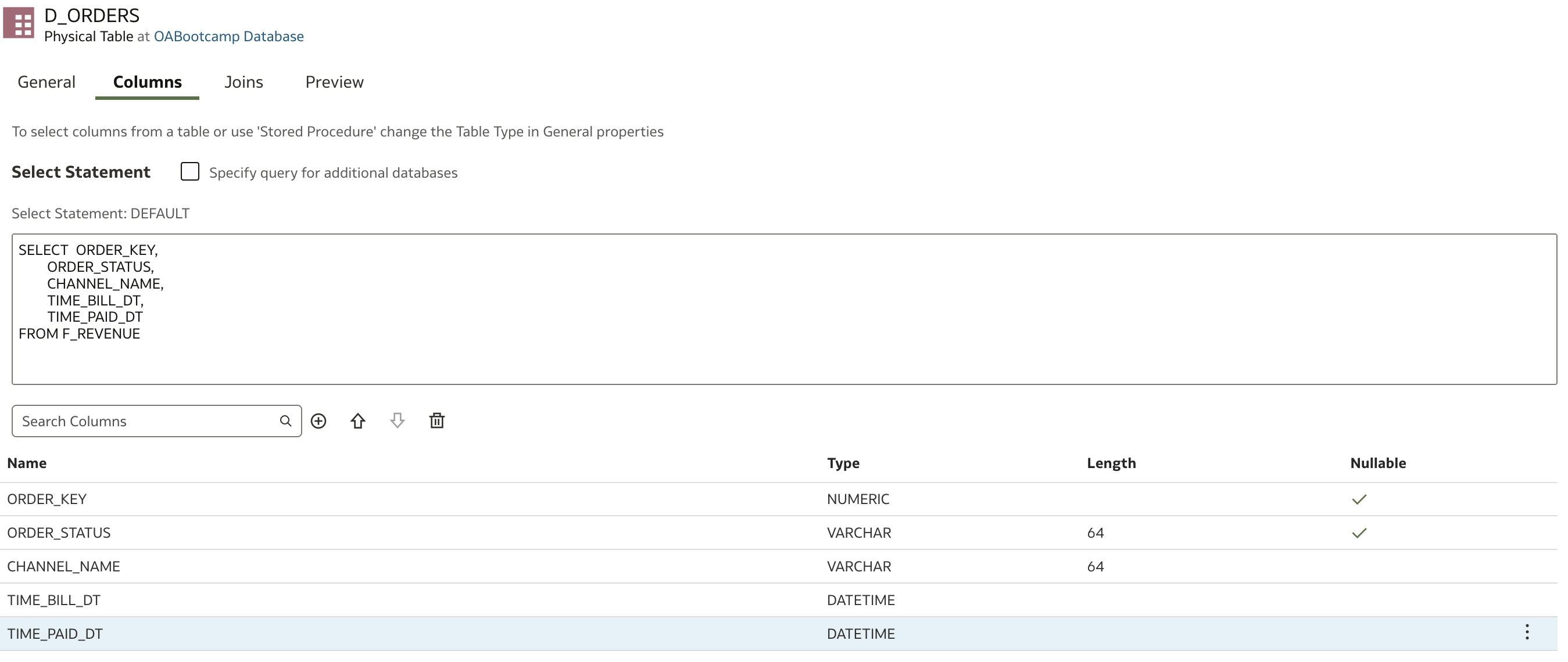
Run a Preview to check your SQL query:
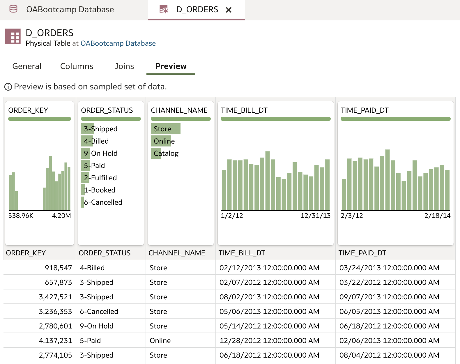
Save your work.
At this point, you have imported several dimension tables, added a fact table, and created a new physical table based on a SQL query.
Next, we will remove columns from the fact table that are neither foreign keys nor measures. By default, fact tables should only contain columns that are either measures or foreign keys relating to dimensions.
In the F_REVENUE fact table, two such candidates are ORDER_STATUS and CHANNEL_NAME. Both columns have been included in the D_ORDERS table and will relate to the fact table using ORDER_KEY, so it is safe to remove them from F_REVENUE.
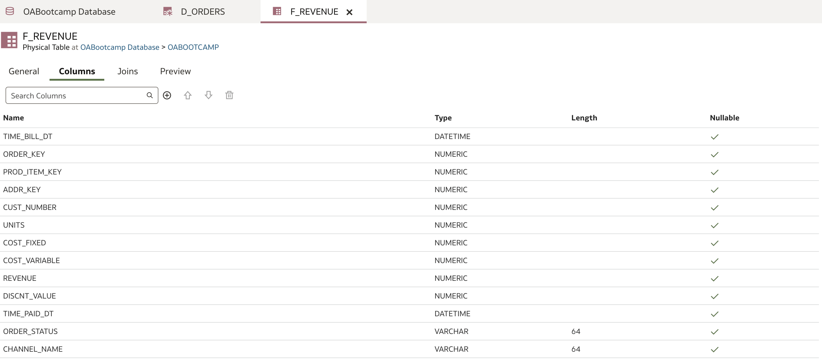
Double-click F_REVENUE in the navigation bar on the left. A new page opens with the definition of F_REVENUE:
Right-click ORDER_STATUS in the column list and select Delete from the menu:
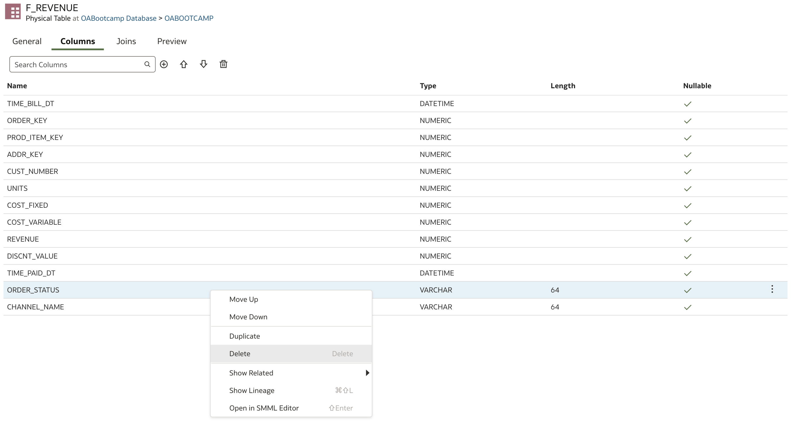
Repeat the deletion for CHANNEL_NAME.
F_REVENUE now contains the following columns:
- Measures
- UNITS
- COST_FIXED
- COST_VARIABLE
- REVENUE
- DISCNT_VALUE
- Foreign Keys
- ORDER_KEY
- PROD_ITEM_KEY
- ADDR_KEY
- CUST_NUMBER
- TIME_BILL_DT
- TIME_PAID_DT
Table Aliases
It is best practice—and often necessary—to create aliases for all physical tables in your database. In some scenarios, as we will see, aliases are required.
Currently, we have six tables in our database: five dimension tables and one fact table. We will create an alias for each, as follows:
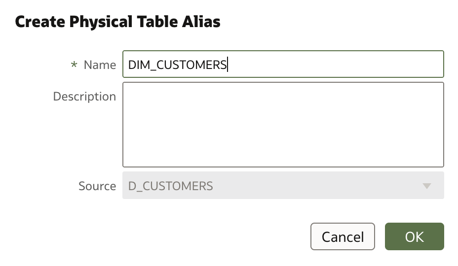
Right-click the desired table name in the Tables list. The table menu opens; select Create Physical Table Alias.
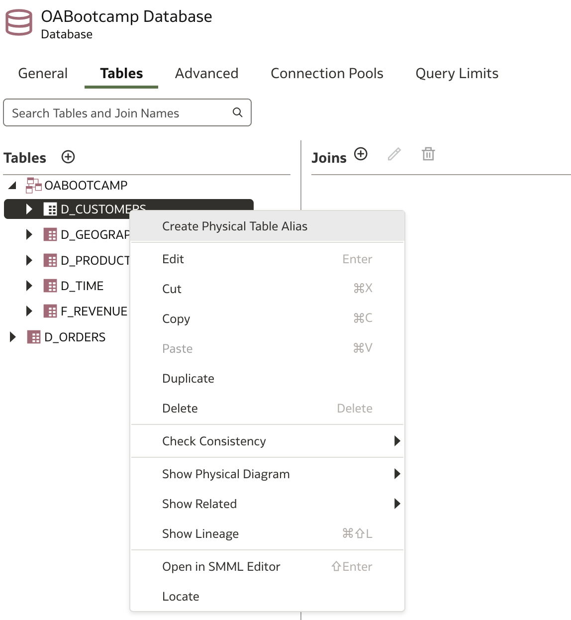
When the Create Physical Table Alias dialog opens, provide a name for the alias.
Repeat these steps for all tables except the dimension table D_TIME.
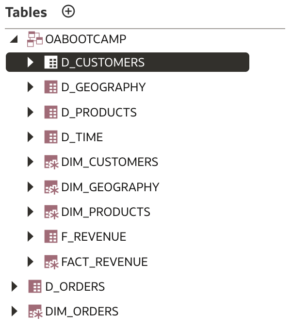
When finished, your Tables list should look like this:
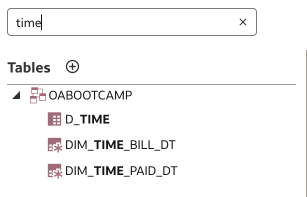
Why treat D_TIME differently? In the fact table, there are two important DATETIME columns:
- TIME_BILL_DT: billing date
- TIME_PAID_DT: payment date
Both relate to the same dimension table, D_TIME. But if only one D_TIME table exists, which date should be joined? Since both are important, the solution is to create two alias tables:
- D_TIME_BILL_DT
- D_TIME_PAID_DT
You do not need separate database tables for each—one time dimension table in your database schema is sufficient. In Oracle Analytics, you resolve this by introducing as many alias tables as needed.
In summary, the following alias tables have been created:
- DIM_CUSTOMERS
- DIM_GEOGRAPHY
- DIM_PRODUCTS
- DIM_ORDERS
- DIM_TIME_BILL_DT
- DIM_TIME_PAID_DT
- FACT_REVENUE
Now we are ready to define Joins.
Joins
Joins are essential because they serve as explicit instructions for the BI Server on how to generate queries. Unless constraints have already been implemented in the database (which is rare in data warehouses), you must create joins manually.
There are two options:
- Use a dialog-driven approach to define and specify each relationship between two tables.
- Use the graphical interface to draw relationships between tables.
Let’s demonstrate the dialog-driven approach first.
Under the Tables tab, there is a Joins section.
To add a new join, click the plus sign (![]() ) next to Joins. The Add Physical Join dialog appears. Define a new join as needed:
) next to Joins. The Add Physical Join dialog appears. Define a new join as needed:
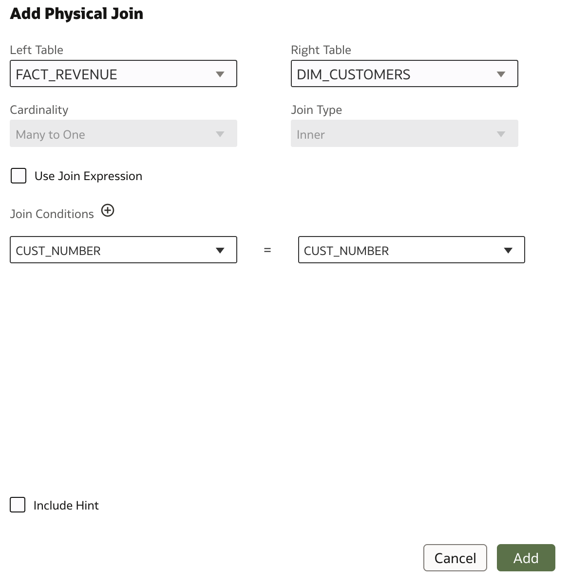
Click Add to save and add the new join to the list.
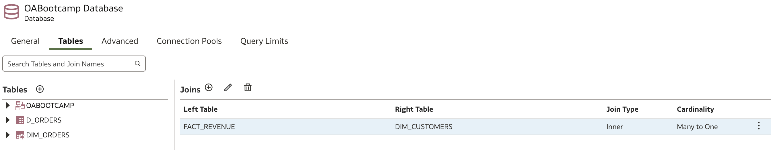
You can continue defining joins one by one, or use the graphical approach.
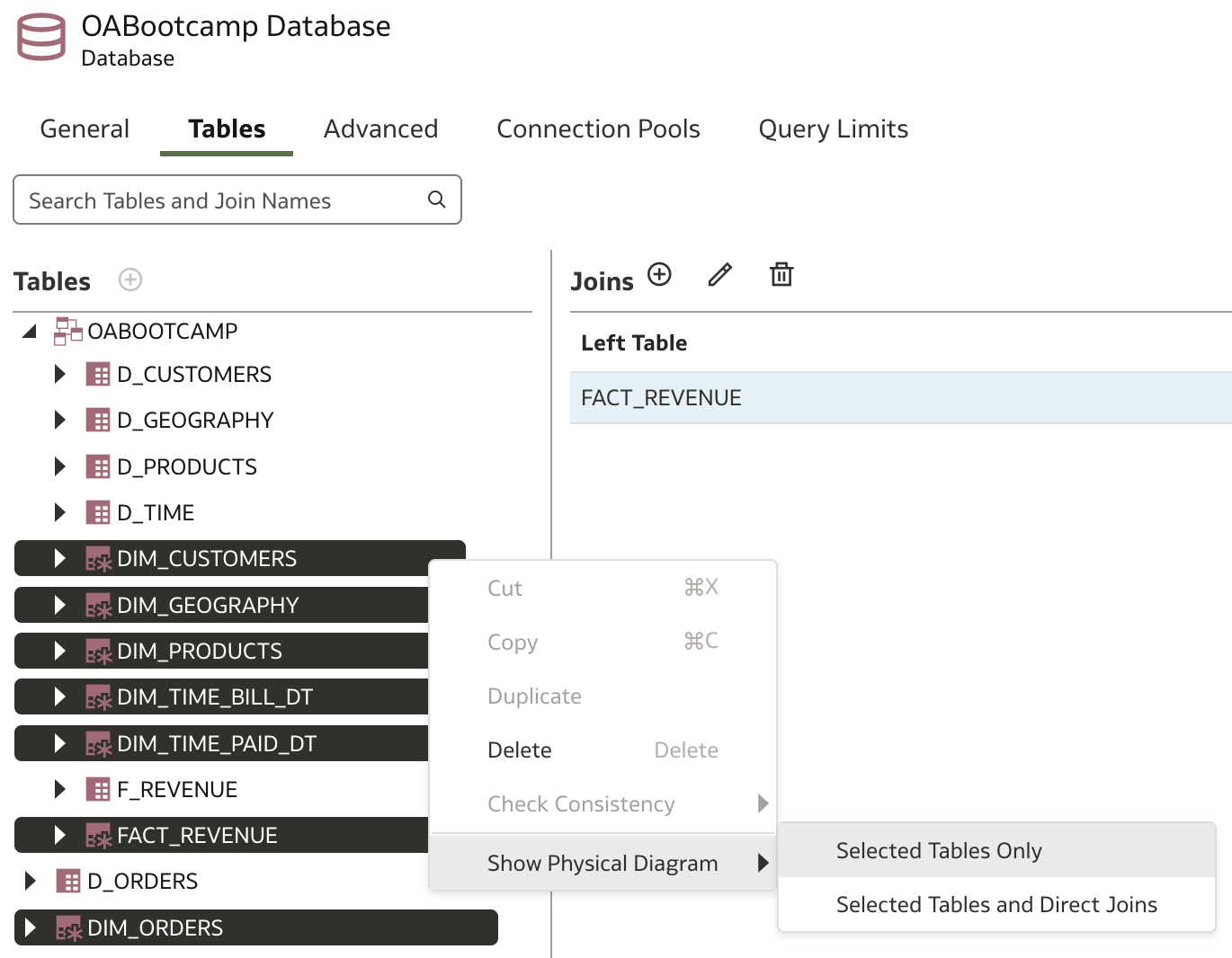
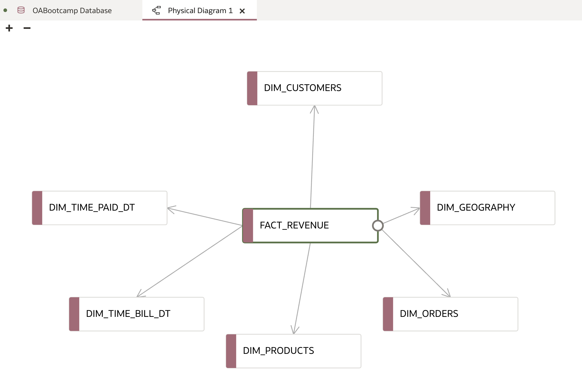
Select all Dim_ and Fact_ tables from the list, right-click, and choose Show Physical Diagram → Selected Tables Only. Alternatively, you can add required tables one by one by dragging and dropping them into the diagram.
In the diagram above, you can see the join created in the previous step. Note the direction of the arrow: it points from the fact table to the dimension table, indicating a Many-to-One relationship (from the fact table’s perspective).
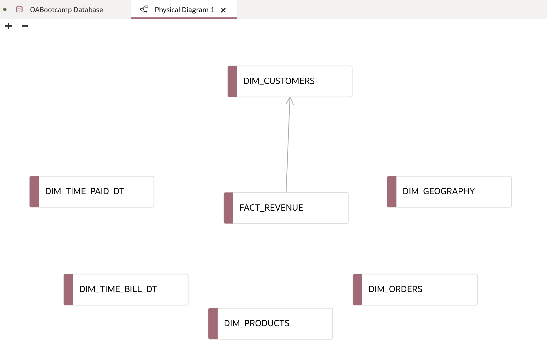
Now, add all other joins. Be mindful of direction—drag from the fact table outward.
When finished, simply close the Physical Diagram 1 tab.
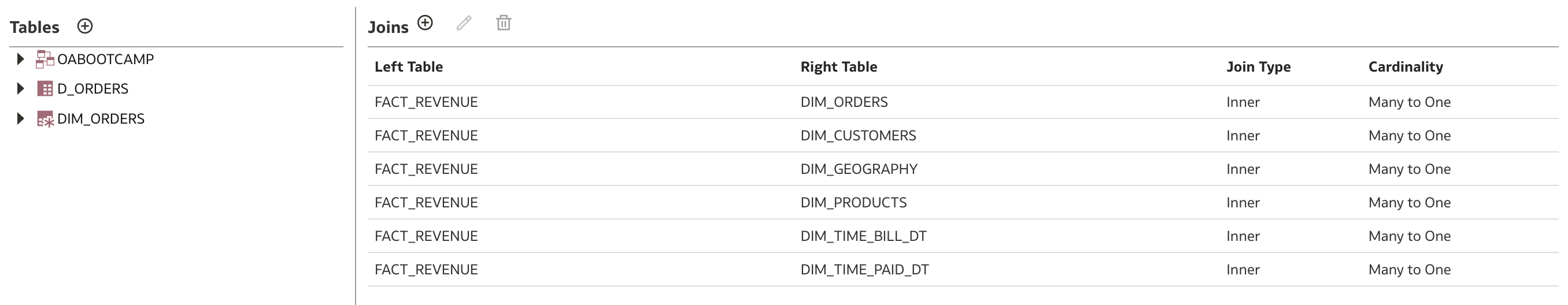
The final joins list should contain the following joins:
Conclusion
In this session, we have built out the Physical Layer: establishing connections, importing tables and views, creating aliases, cleaning up the fact table, and defining joins. This critical groundwork ensures that the raw data is ready for logical modeling and business transformation. With a well-prepared Physical Layer, you are now ready to move on to the next phase: designing the Logical Layer (also known as the Business Layer), where business meaning and usability come to the forefront.