Semantic Model Series: 4. Logical Layer

Understanding the Logical Layer in Oracle Analytics

The Logical Layer, also known as the Business Layer, is a central component in Oracle Analytics' Semantic Model (RPD). Its primary role is to bridge the gap between complex physical data structures and the business-friendly views that users interact with during analysis. By abstracting, organizing, and enriching data, the Logical Layer enables consistent, optimized, and meaningful insights for end users. In this guide, you'll learn about the key features of the Logical Layer, including how it abstracts data, defines logical tables and columns, manages relationships and joins, handles aggregations and calculations, and supports advanced data scenarios. We'll also walk through the practical steps of building a logical model, working with facts and dimensions, and preparing your model for the next stage—the Presentation Layer.

Key Features of the Logical Layer

The Logical Layer delivers several core capabilities that make business analytics possible and efficient. Let's break these down into consistent, clearly labeled subsections:

Abstracting Data

• Business-Friendly Abstraction: The Logical Layer maps complex, normalized physical database schemas into intuitive business models. End users interact with familiar entities and attributes, without needing to understand physical joins, foreign keys, or source complexities.
• Single Source of Truth: By encapsulating business logic and definitions, the Logical Layer ensures consistency across dashboards and reports.
• Performance Optimization: Through abstraction and metadata-driven design, the Logical Layer helps optimize SQL generation and query execution.

Logical Tables & Columns

• Logical Tables: These represent business entities such as Customer, Sales, or Product. Logical tables can aggregate data from one or more physical sources.
• Logical Columns: Columns in logical tables can directly map to physical columns or be defined as calculated expressions, supporting both simple and advanced business logic.
• User-Friendly Naming: Tables and columns can be renamed to align with business terminology, making models easier for users to understand.

Relationships & Joins

• Logical Joins: The Logical Layer defines business relationships between entities (e.g., Customers have Orders). Unlike physical joins, logical joins exist at the metadata level and guide the generation of optimized queries.
• Flexible Join Management: Logical joins can be created and managed independently of the underlying physical join definitions, allowing for more intuitive data relationships.

Aggregation & Calculations

• Aggregation Rules: Default aggregation methods (SUM, AVG, COUNT, COUNT DISTINCT, etc.) can be set for each measure, ensuring correct roll-up behavior in analyses and dashboards.
• Level-Based Measures: Measures can be designed to aggregate differently depending on the level of a hierarchy (e.g., monthly vs. yearly revenue).
• Derived Metrics & KPIs: The Logical Layer supports the creation of calculated columns and key performance indicators, embedding business rules directly into the model.

Advanced Data Handling

• Multiple Data Sources: Logical tables and columns can draw from multiple physical sources, even across different systems (e.g., combining relational tables with OLAP cubes).
• Data Filters: Row-level and column-level security, as well as explicit and implicit data filtering, can be implemented to control data visibility and access.
• Hierarchies: Only dimension tables can have hierarchies, which enable drill-down and roll-up functionality for analysis.

Create a new Logical Model

To start with, navigate to Logical Layer tab.

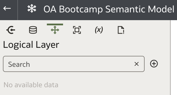
Currently, there are no logical models available. Let's create one.

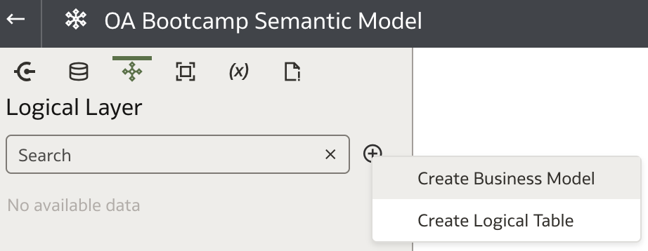
As usual, click the plus icon () to open the menu. Select Create Business Model.

The Create Business Model dialog opens. Provide a name for the logical model.

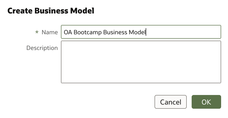
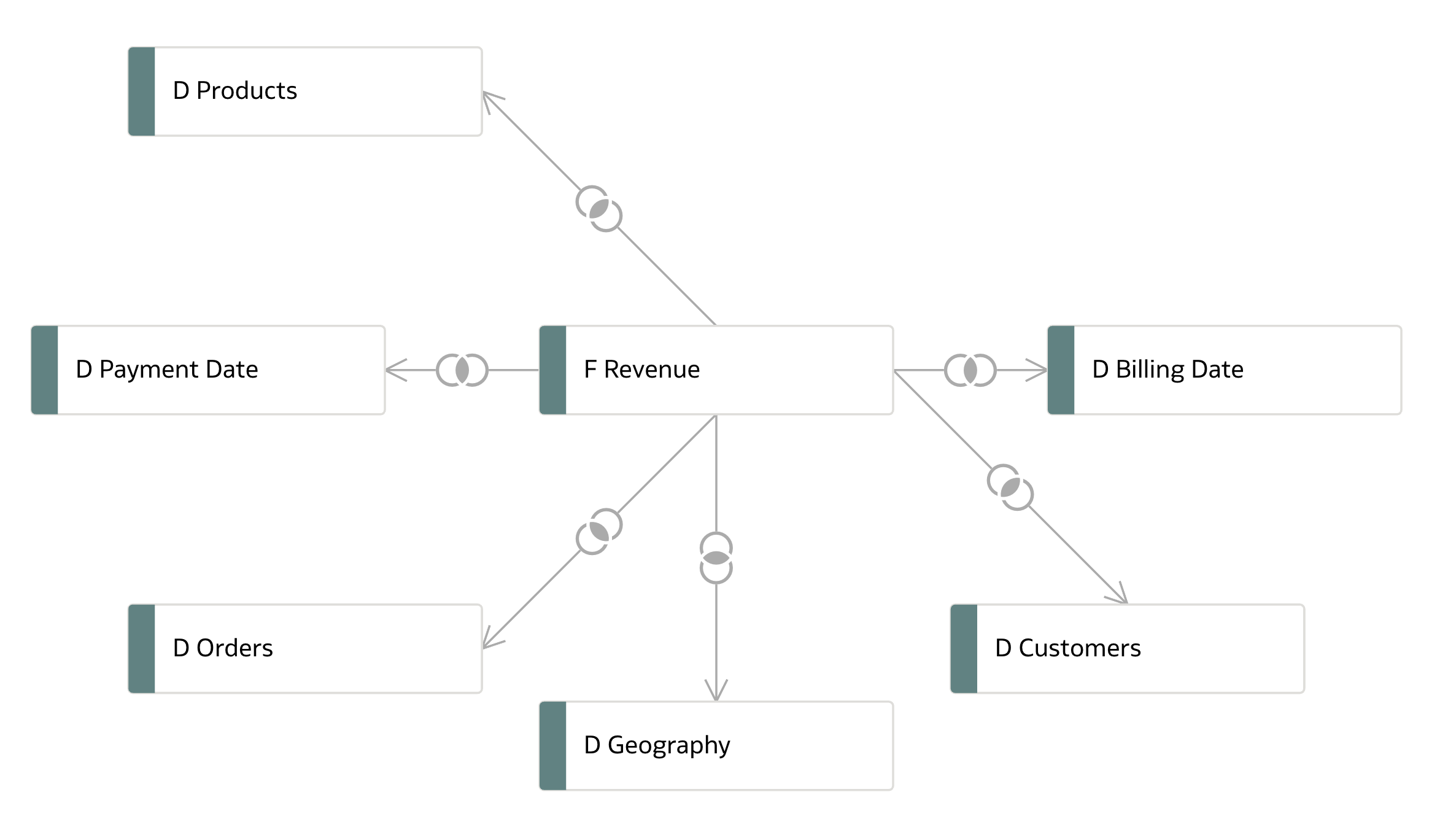
Click Ok to create a new business model. The main canvas consists of three areas in the Logical Layer tab:

• Facts
• Dimensions
• Logical Joins

Next, we need to import tables created in the Physical Layer, separating them into facts and dimensions. Joins will be created manually.

There are two main ways to import and create logical tables (facts and dimensions). One is by using the plus icon (). We'll start with this option and explore the other later.

Let's add the fact table FACT_REVENUE to the logical model.

Facts

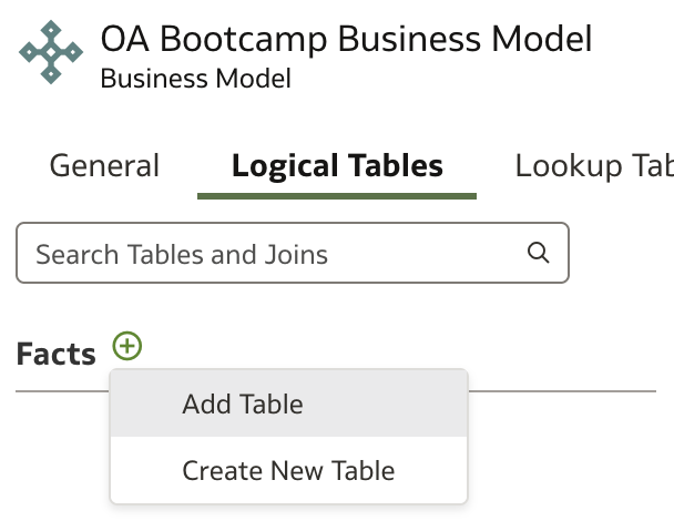
Click the plus icon () next to Facts. A menu with two options appears. Add Table lets you import a table directly from the Physical Layer, while Create New Table allows you to build logical tables step by step. All columns must eventually be mapped to physical columns or defined as calculations.

For now, select Add Table.

The Select Fact Table dialog appears. Search for and select the FACT_REVENUE table.

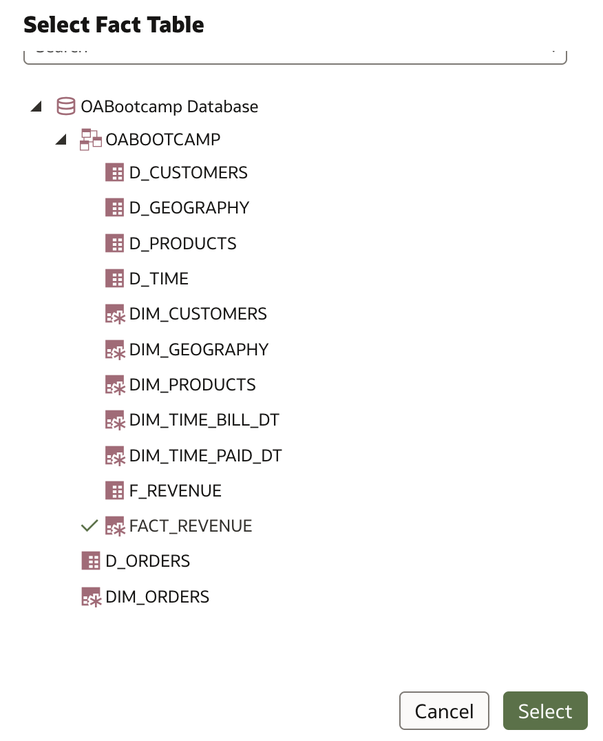
FACT_REVENUE is now listed under Facts.

Double-click the FACT_REVENUE fact table to explore its properties and make adjustments.

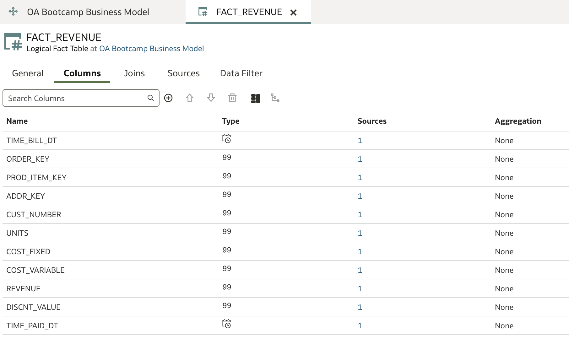
There are five tabs for managing a logical fact table (note: we use logical to distinguish these tables from physical tables):

• General: Rename tables and columns to be more business-user friendly. This can also be done in the Presentation Layer, but is often handled here.

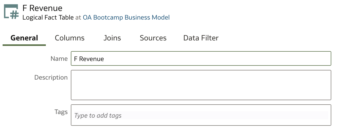
We will return to the Columns tab for detailed explanations, but note that here you can rename columns, remove or hide them, and set default aggregations.

• Joins: Create and manage logical joins between tables. These are based on physical joins, but are managed at the logical level.

• Sources: Oracle Analytics' Semantic Model is especially strong in managing multiple data sources. Logical tables and columns can have multiple sources, even across different systems. For example, a logical column may be sourced from both a detailed relational table and an aggregated OLAP cube.

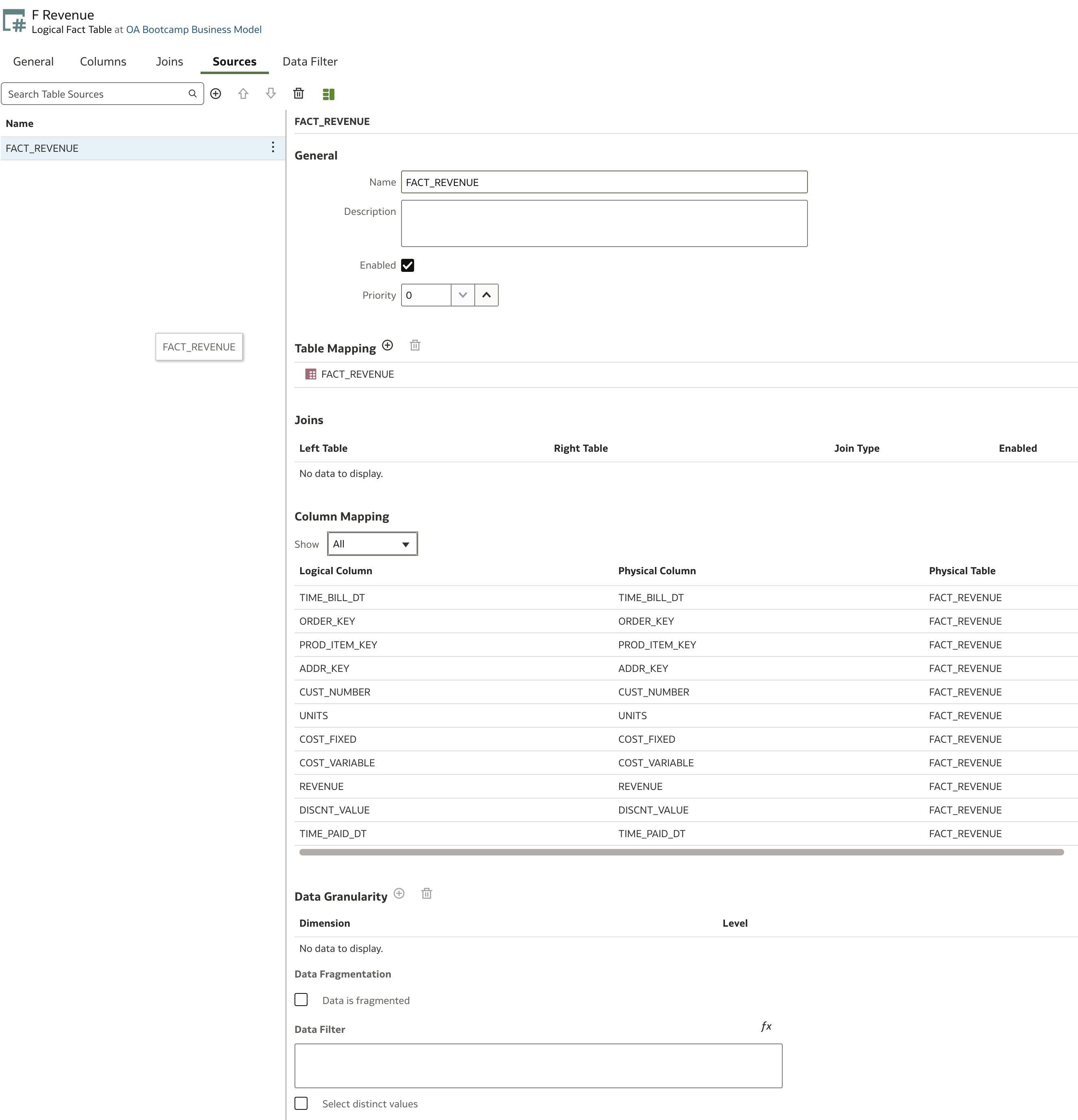
In the screenshot above, FACT_REVENUE has one Table Mapping, no Joins yet, and visible Column Mappings.

• Data Filter: Apply explicit and implicit data filters, such as implementing row-level security based on user attributes.

Let's return to the Columns tab.

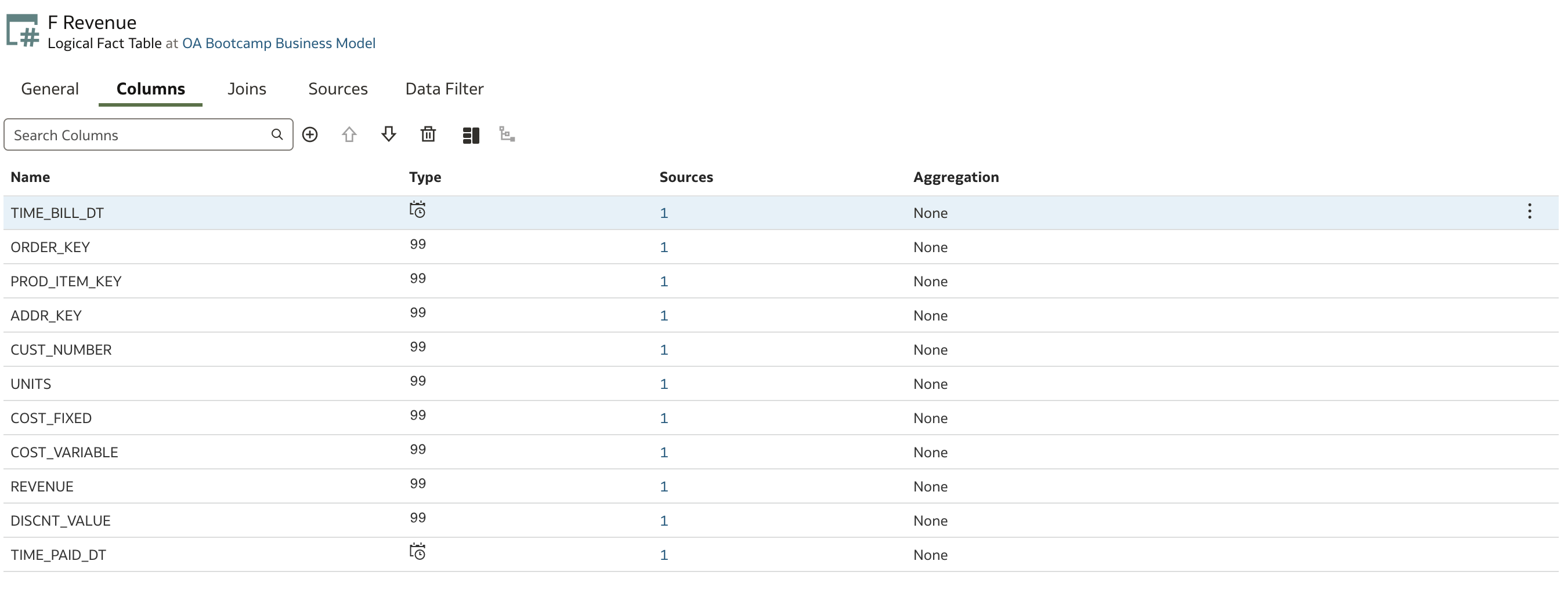
Fact tables typically contain two types of columns:

• Measures (quantitative data)
• Foreign keys (references to dimensions)

You should specify a default aggregation for each measure. Normally, you might remove foreign key columns, but sometimes these can be used as measures (for example, counting distinct orders).

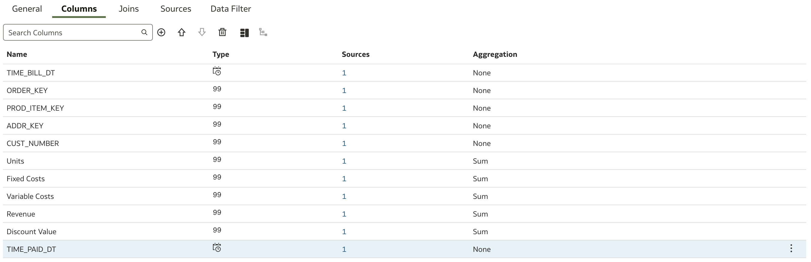
Scroll to the REVENUE column. Double-click the column name to edit it. Make two adjustments:

• Rename REVENUE to Revenue
• Set Aggregation to Sum

Repeat this process for other obvious measures such as UNITS, COST_FIXED, COST_VARIABLE, and DISCNT_VALUE.

Sometimes, you may need to count distinct values such as the number of customers, products sold, or orders. You can use foreign key columns for this purpose by assigning appropriate aggregation rules.

For each column, you can review its details by clicking the Details icon:

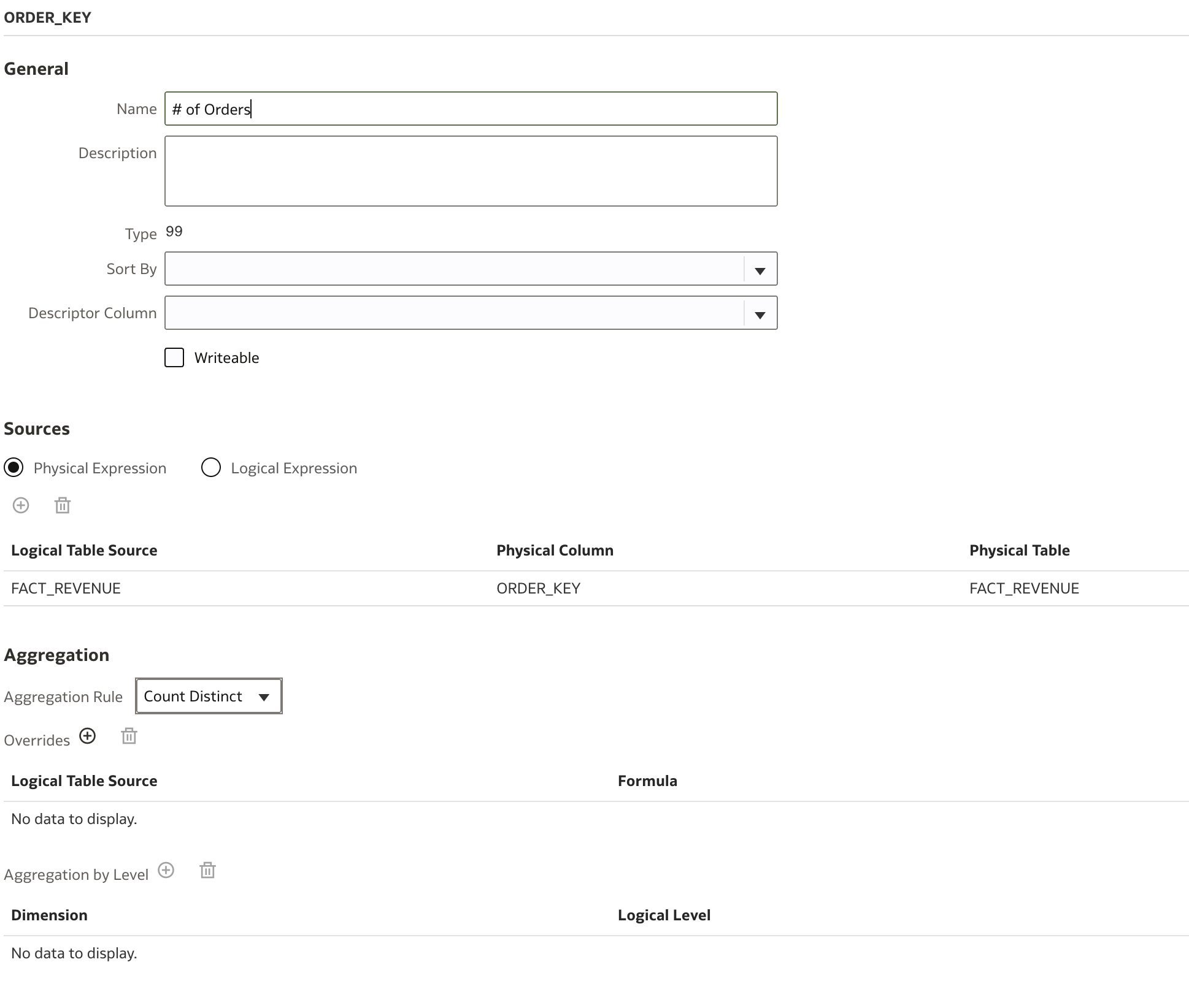
Scroll to the ORDER_KEY column, select it, and click the Details icon.

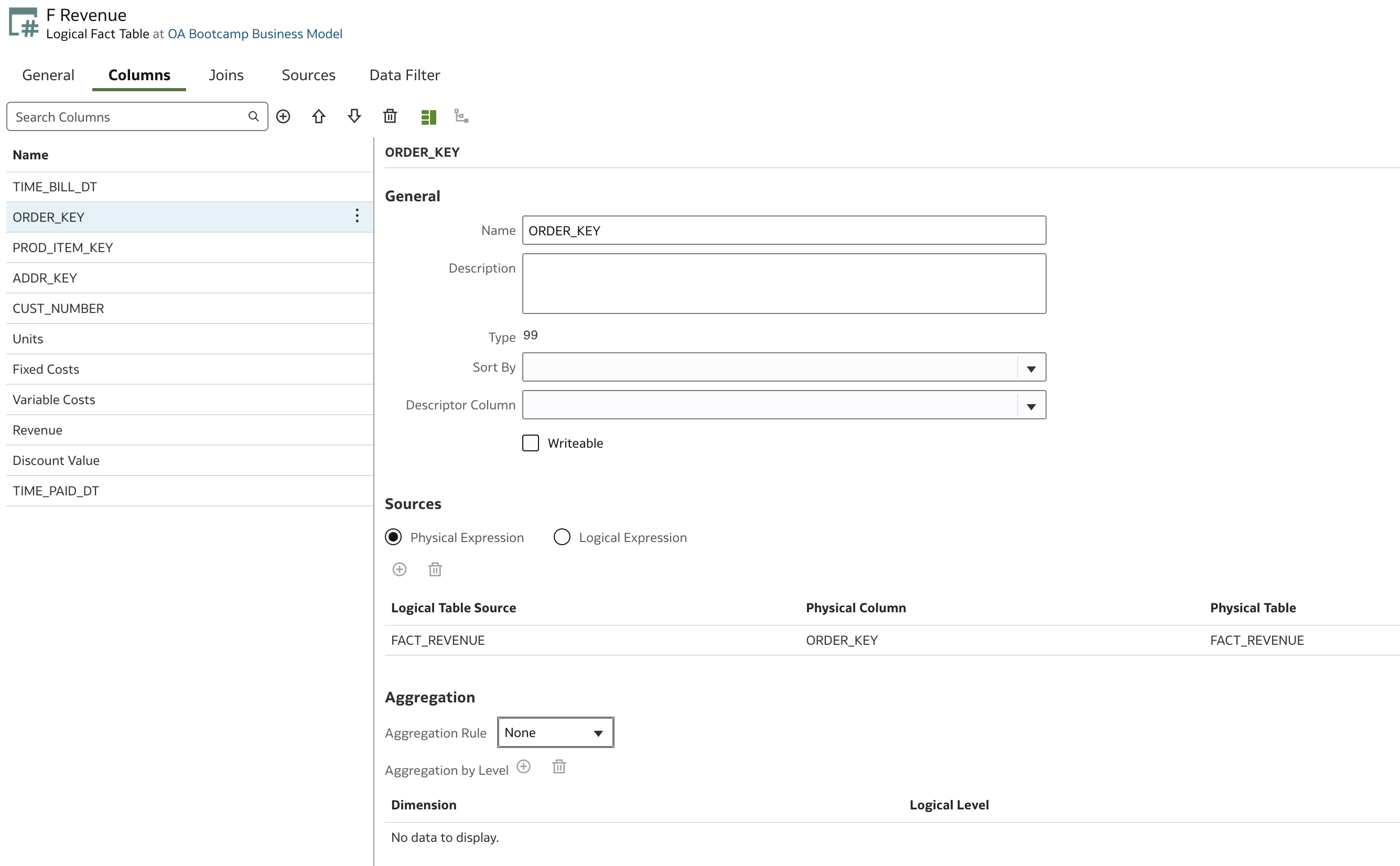
We'll use this column to count distinct orders. Rename the column to # of Orders and set the default Aggregation Rule to Count Distinct.

You can update other foreign key columns similarly if needed. Leave unnecessary columns unchanged.

We have made minimal updates to our fact table. We'll revisit facts later, but now let's move on to dimensions.

Dimensions

Dimension tables are generally managed similarly to facts, but with some important differences.

Let's add our first dimension table manually for learning purposes. Click the plus icon () next to Dimensions.

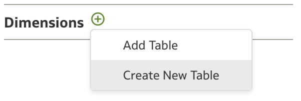
This time, select Create New Table to build a logical table from scratch. The Create Logical Table dialog opens.

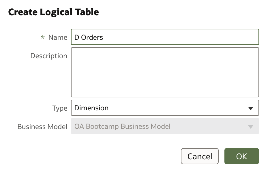
Provide a name and click Ok. The new logical table page opens with no columns, so you'll need to add some.

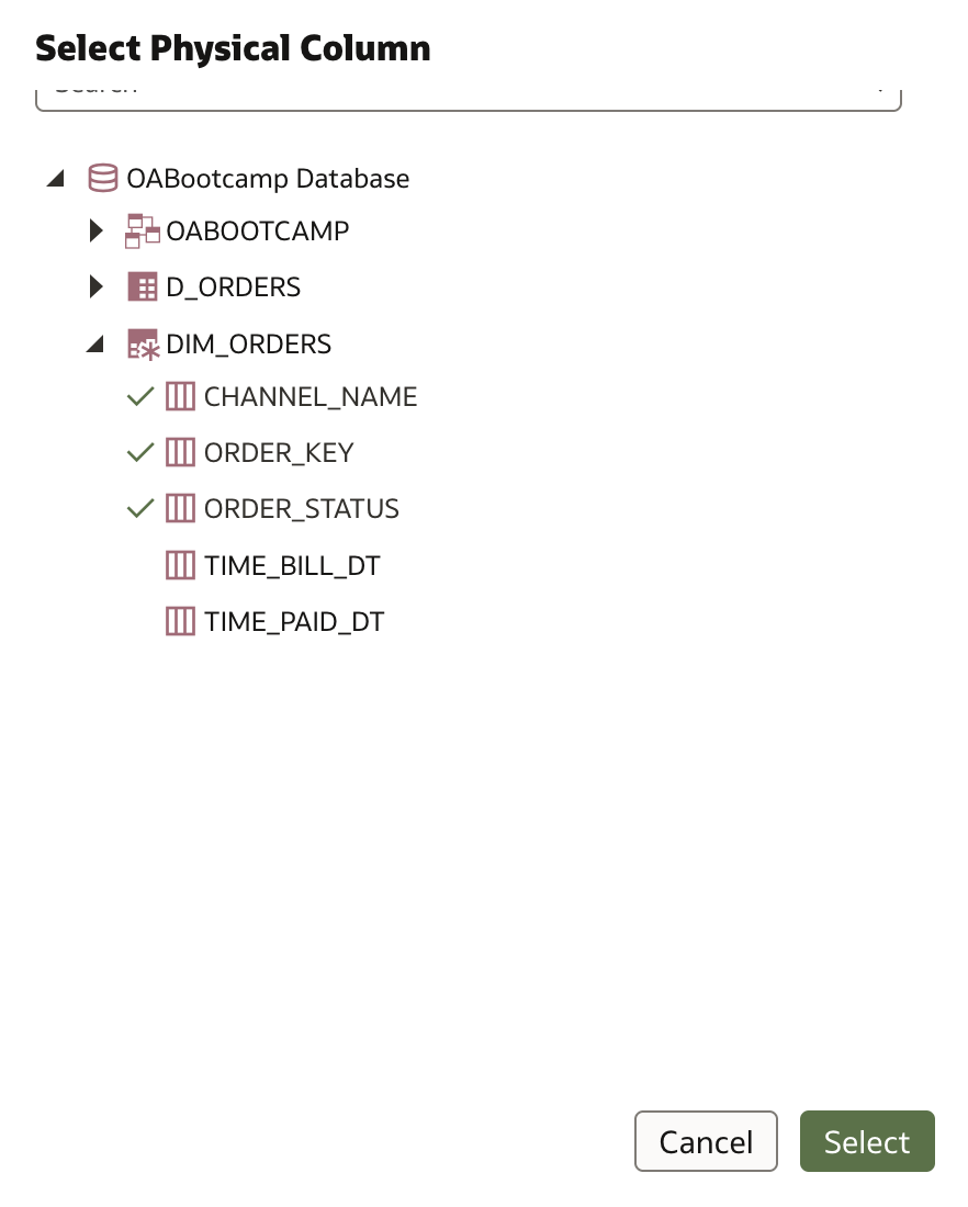
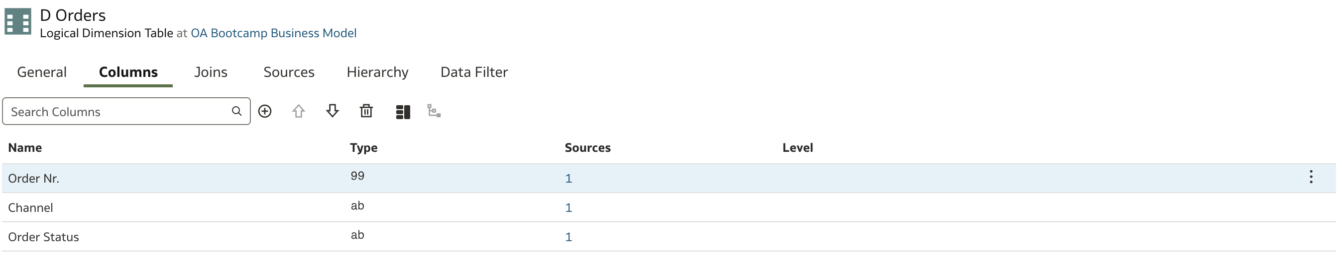
Click the plus icon and select Add Physical Column from the menu.

In the Select Physical Column dialog, select ORDER_KEY, ORDER_STATUS, and CHANNEL_NAME from DIM_ORDERS.

Rename the columns as follows:

Let's briefly review the tabs available for dimension tables:

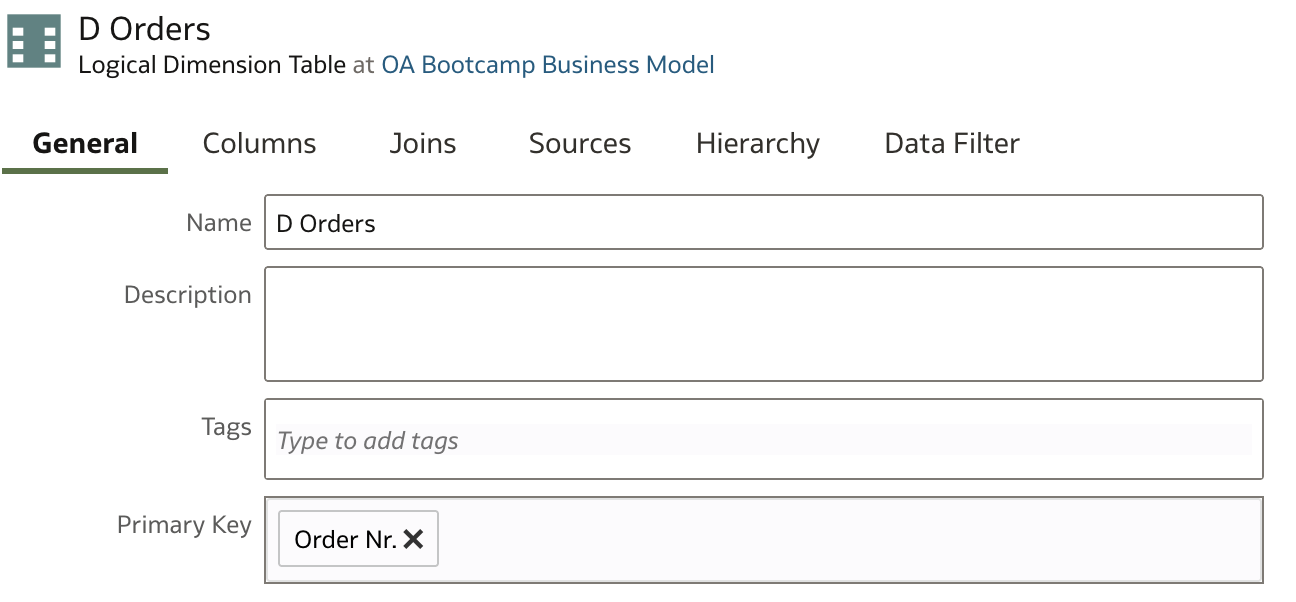
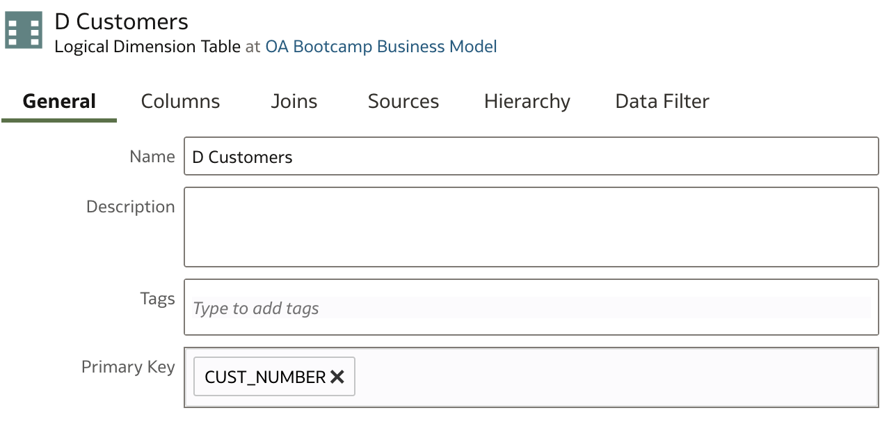
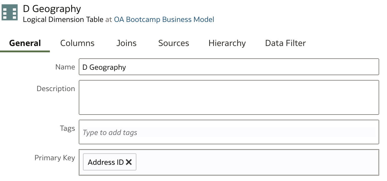
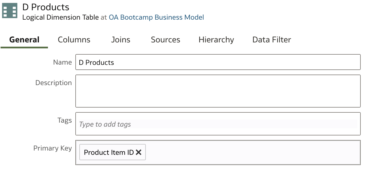
• General: Similar to facts, except you can define the Primary Key here:

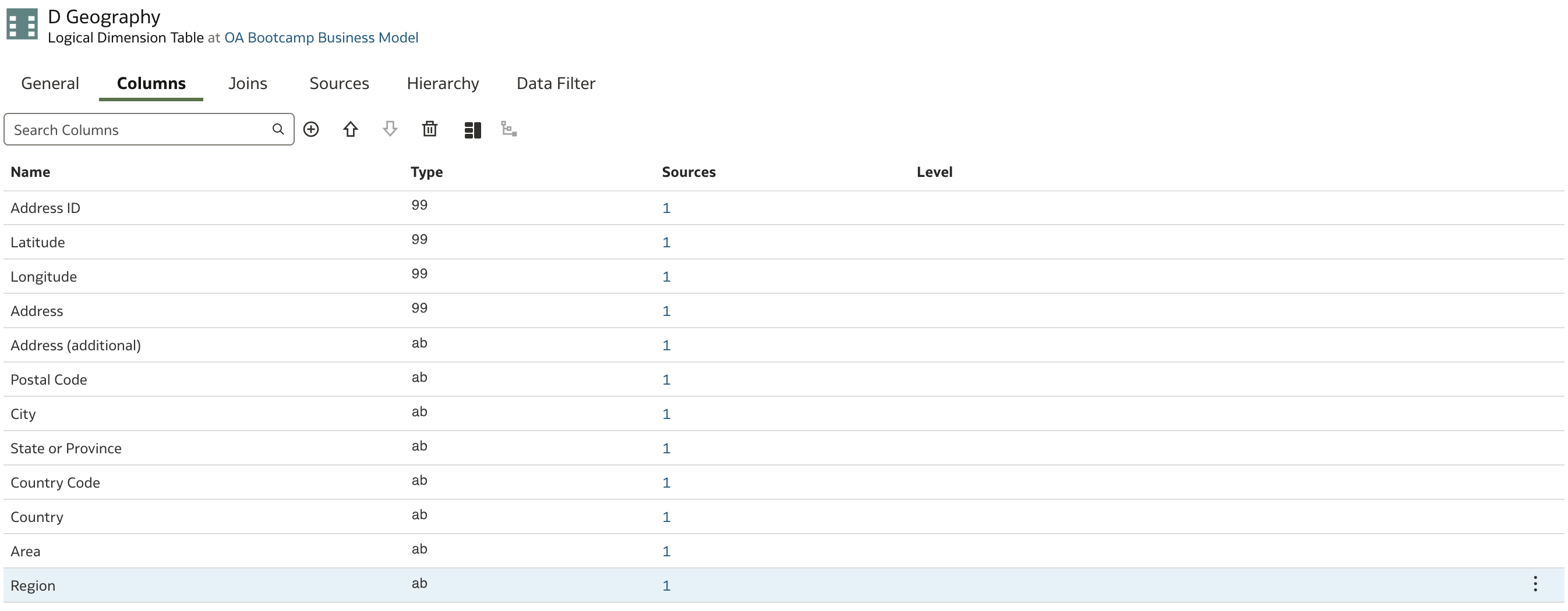
The Columns, Joins, Sources, and Data Filter tabs function the same as for facts.

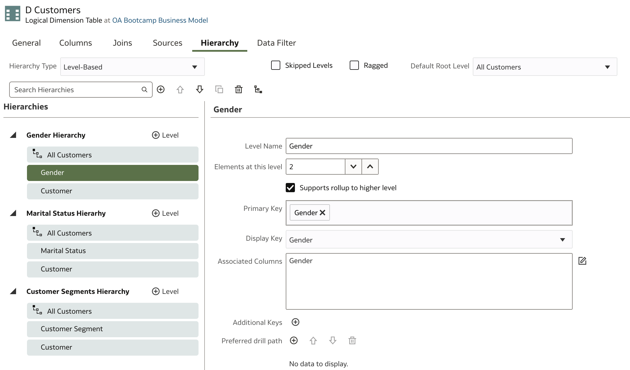
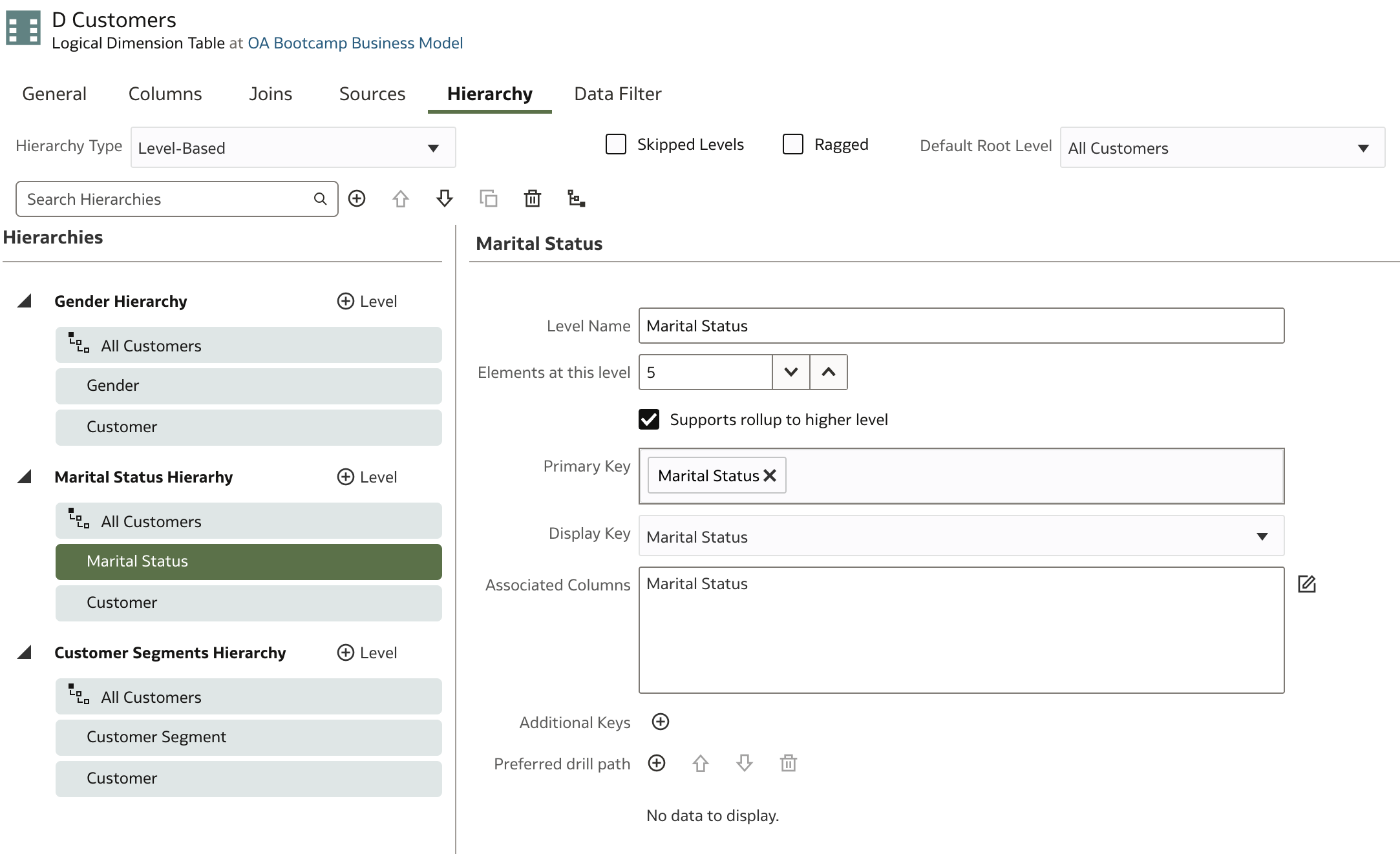
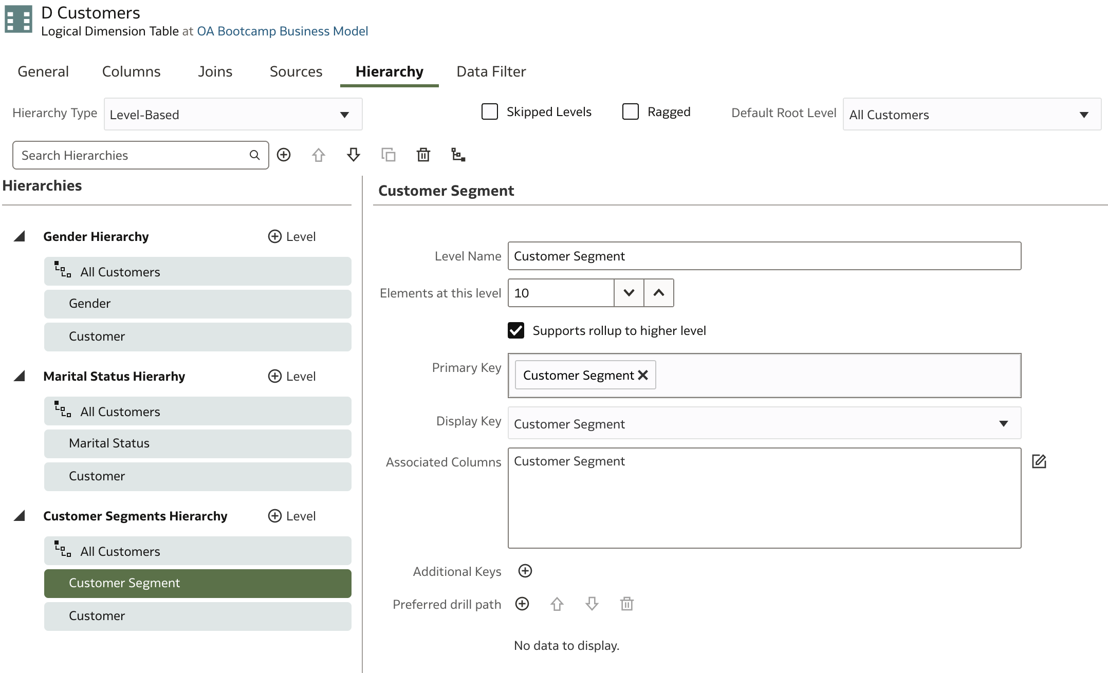
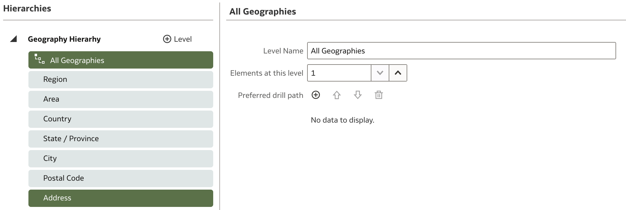
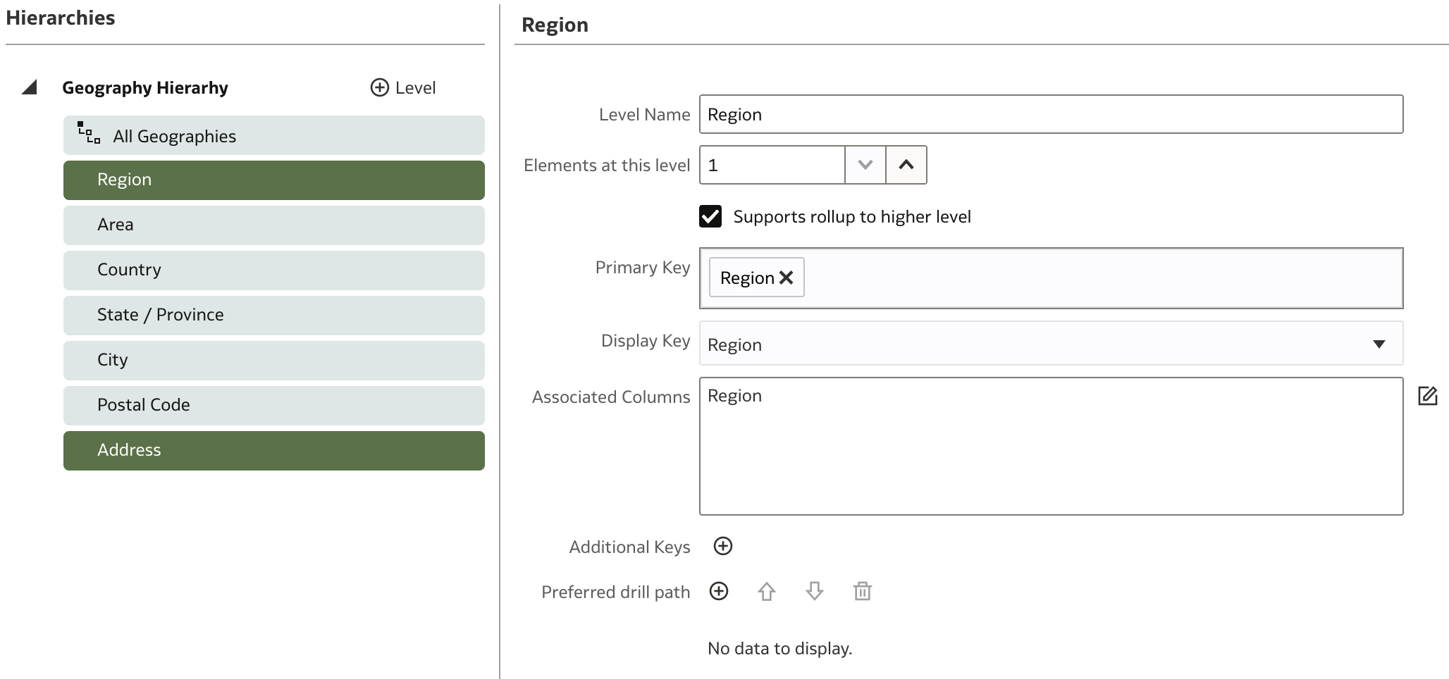
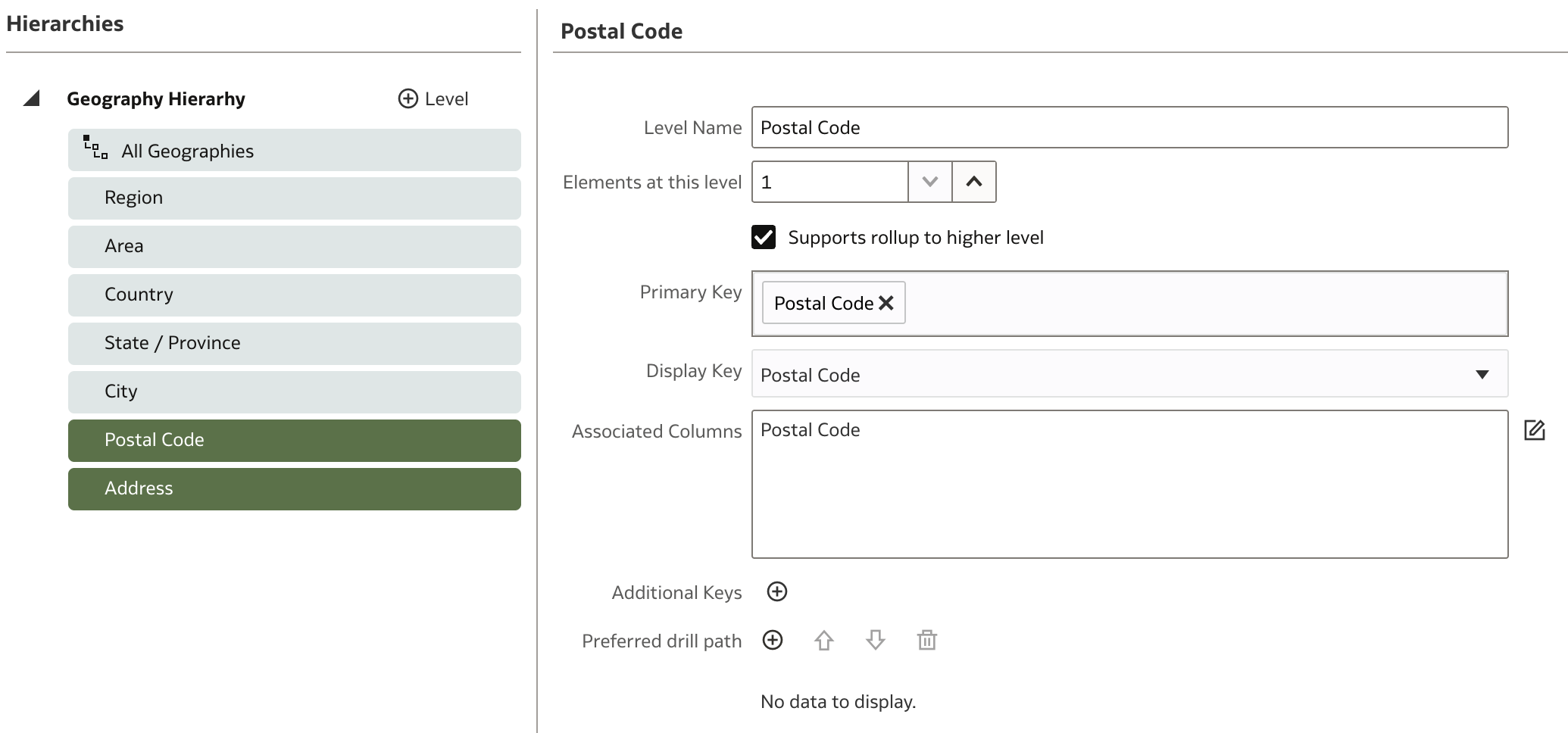
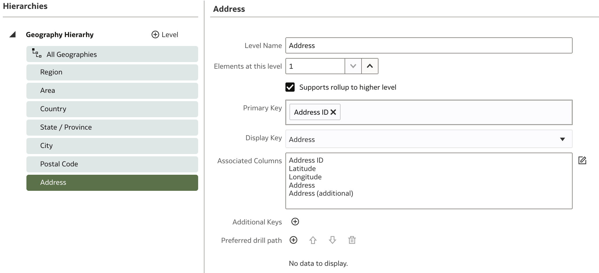
• Hierarchy: Unique to dimensions, only dimension tables can have hierarchies. Hierarchies are essential for data presentation and aggregation, enabling users to drill down or roll up data as needed. Multiple hierarchies can be created based on different analysis needs.

This table has few attributes, so its hierarchies will be simple. For example, you might aggregate and present revenue by channel or by order status—both are candidates for hierarchies.

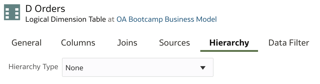
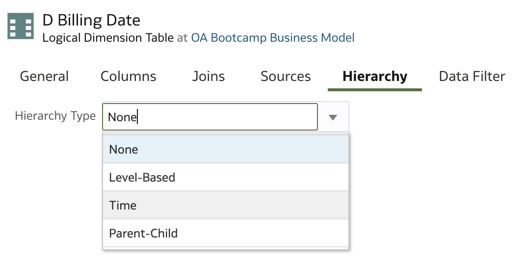
Navigate to the Hierarchy tab. There are no hierarchies yet, and Hierarchy Type is set to None.

There are three Hierarchy Types:

• Level-Based
• Parent-Child
• Time

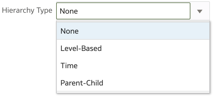
The D Orders dimension is Level-Based, so select this value.

The default hierarchy is displayed.

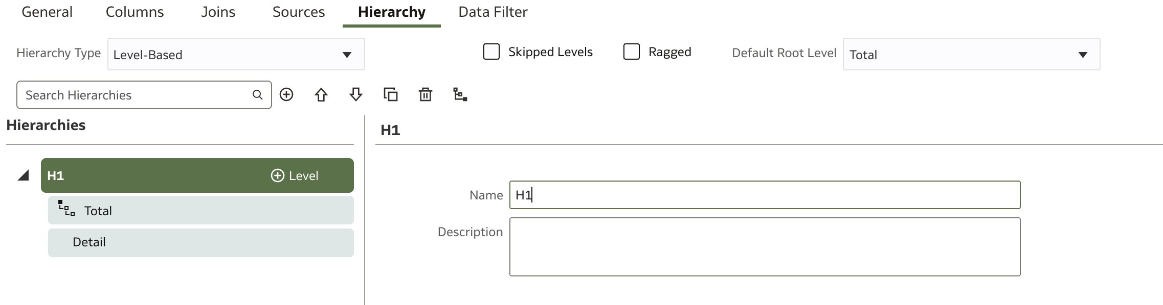
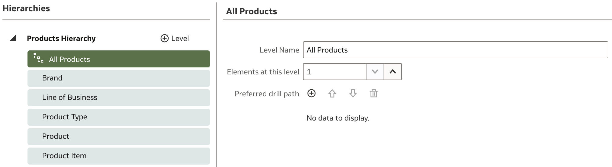
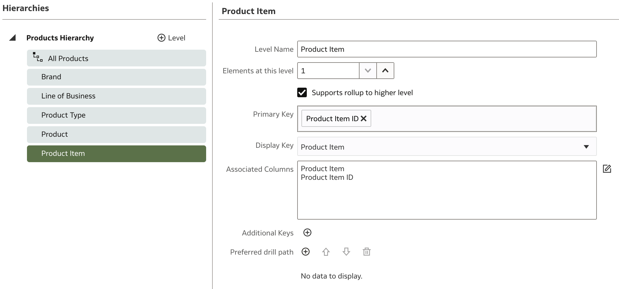
One default hierarchy, H1, has two levels: Total and Detail. You can rename these and add intermediate levels as needed:

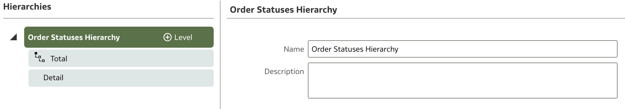
• Click H1 in Hierarchies and rename it to Order Statuses Hierarchy.

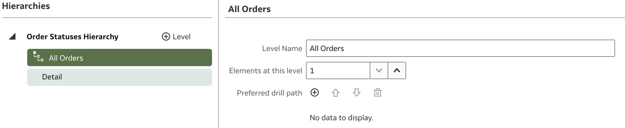
Click Total (the highest aggregation level) and rename it to All Orders. The total level is present in all hierarchies.

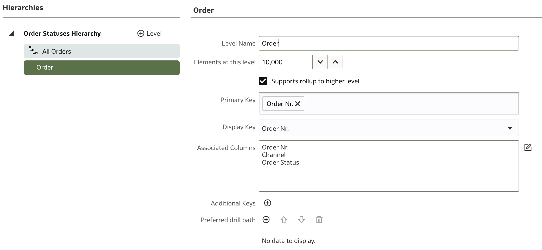
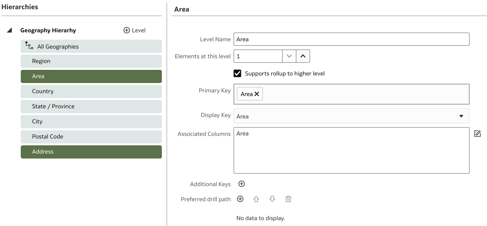
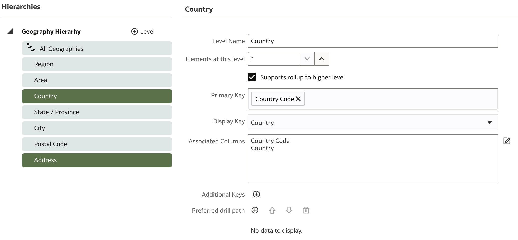
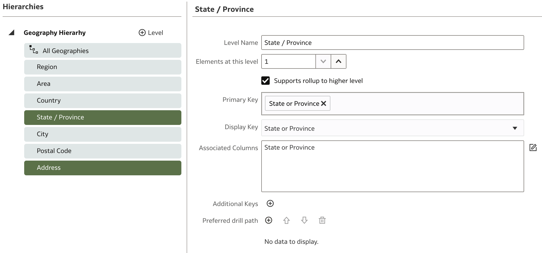
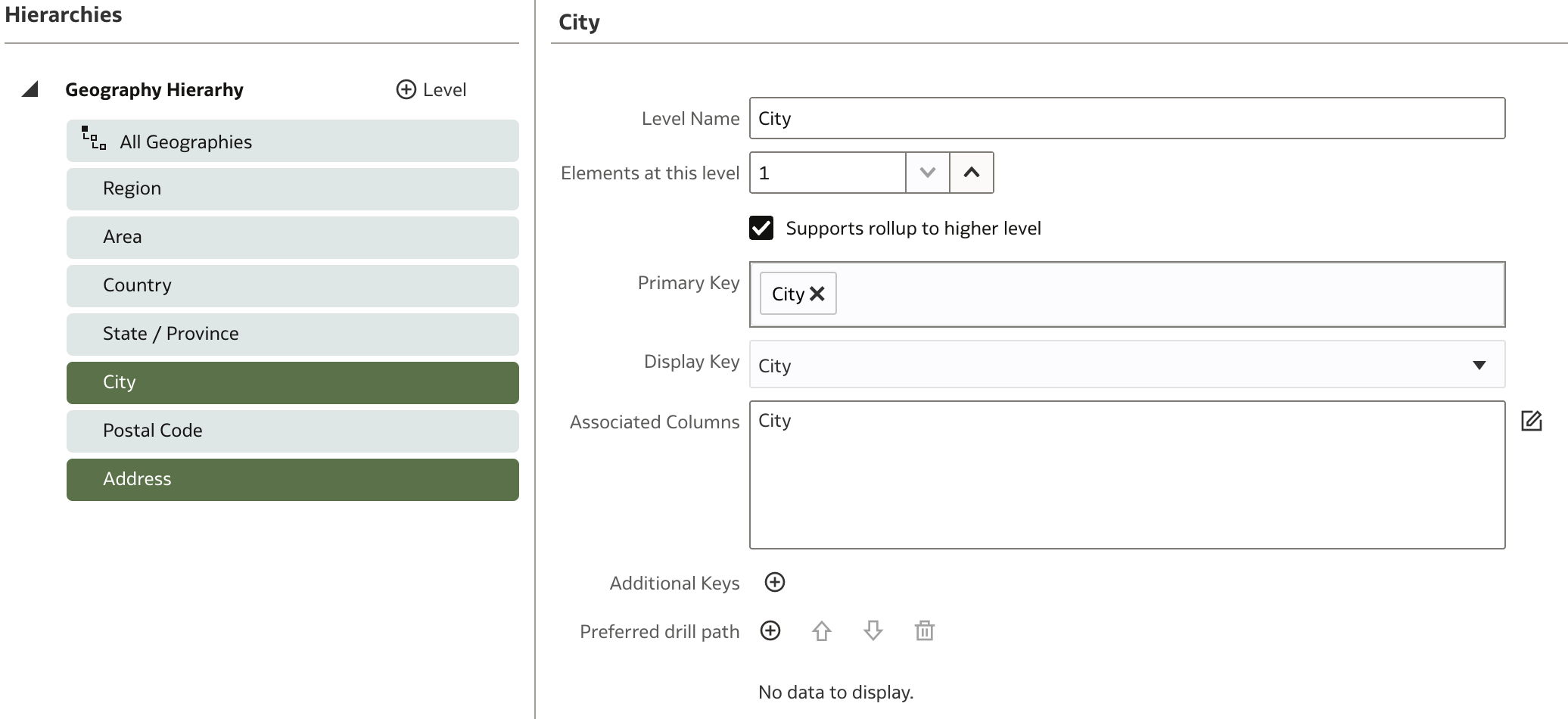
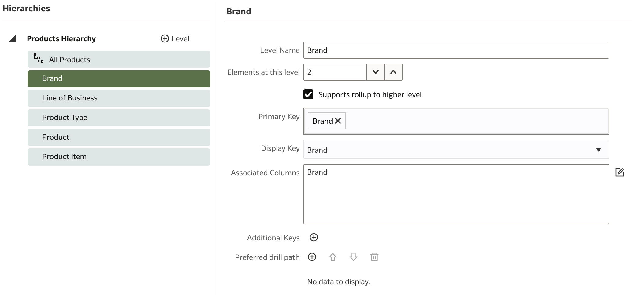
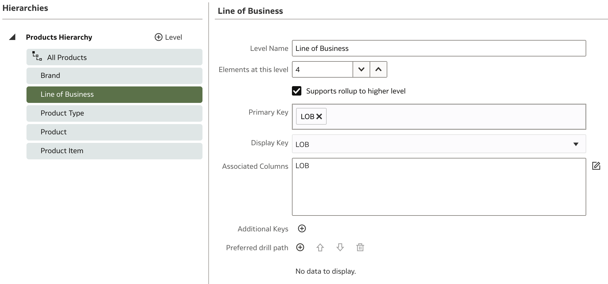
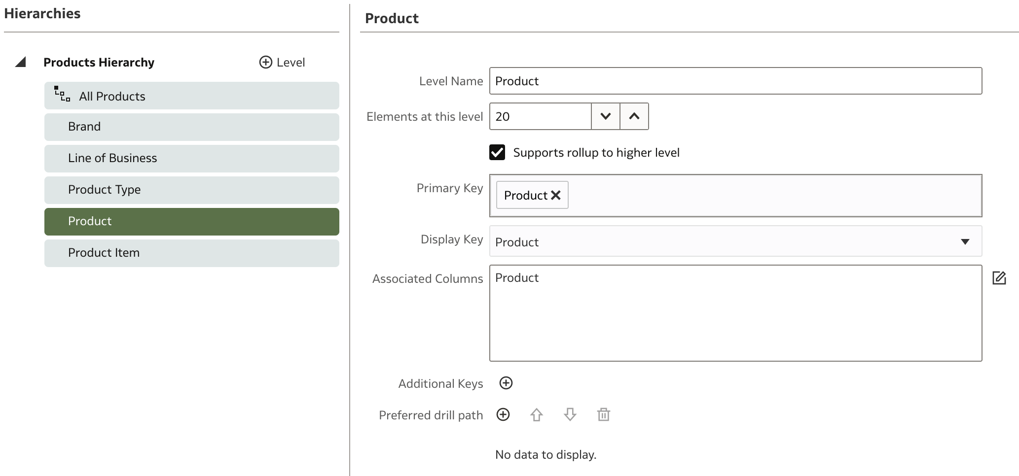
Click Detail (the lowest granularity level) and rename it to Order. It's helpful to specify the number of elements at each level to optimize query performance. Ensure the "rollup" option is checked. Set the primary key and display key as Order Nr.. Leave the associated columns as they are for now.

To add a new level between Total and Detail:

• Click All Orders and then click Level next to the hierarchy.

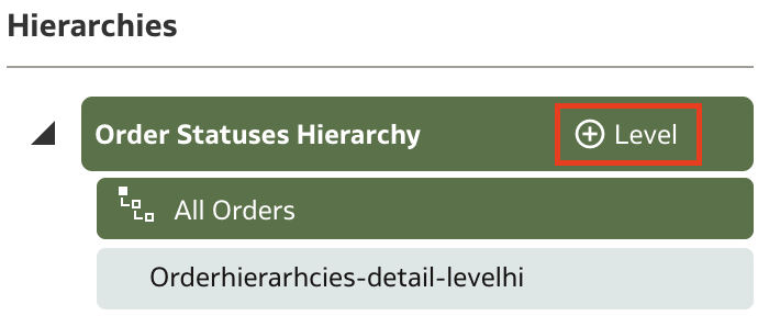
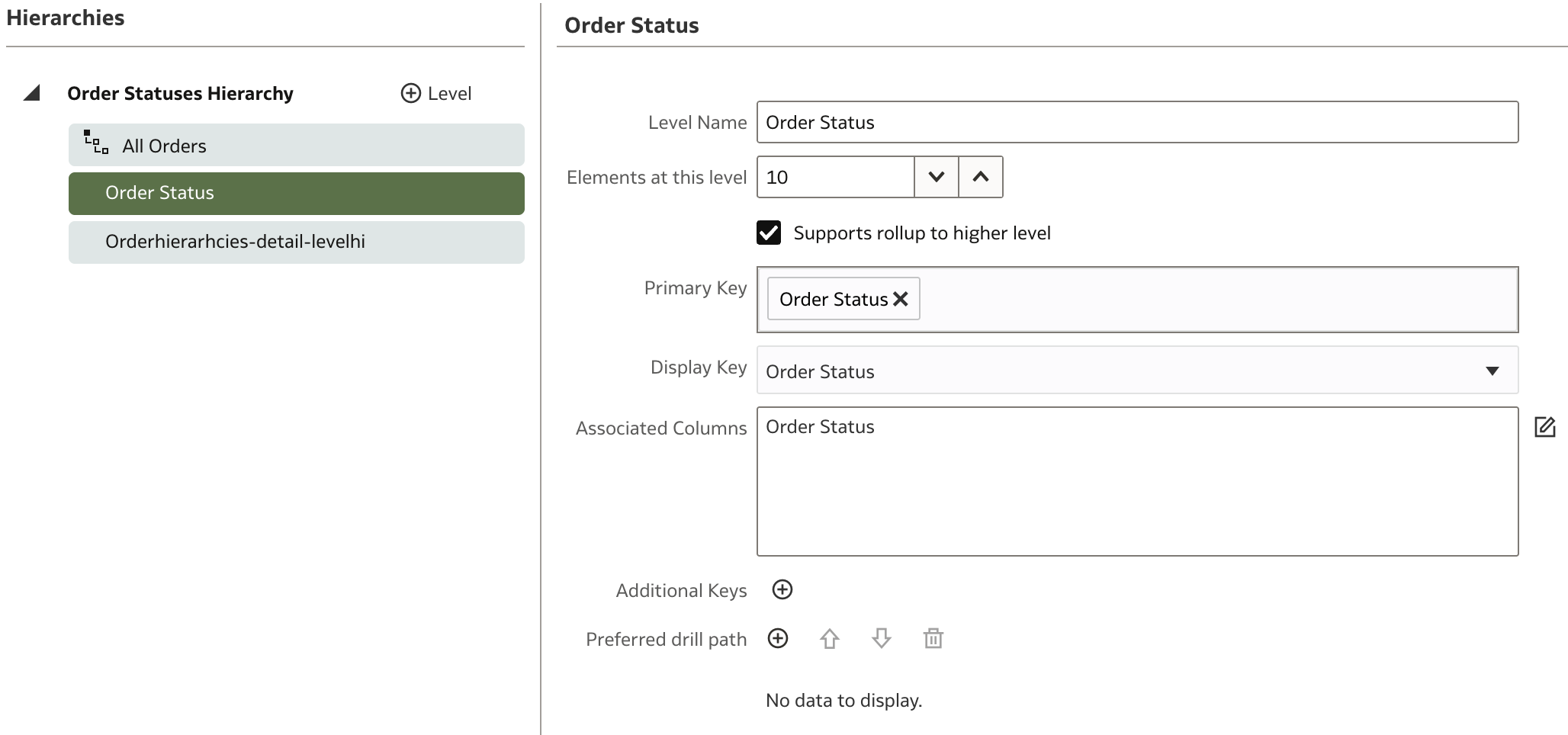
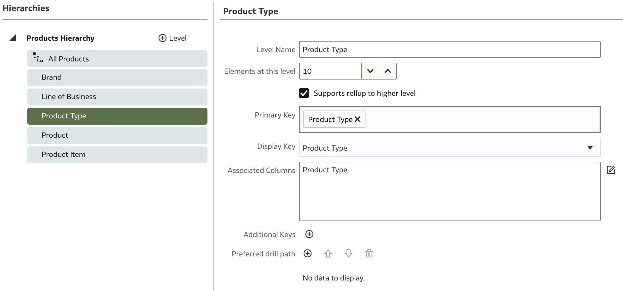
This adds a new level between Total and Detail. Provide the necessary details.

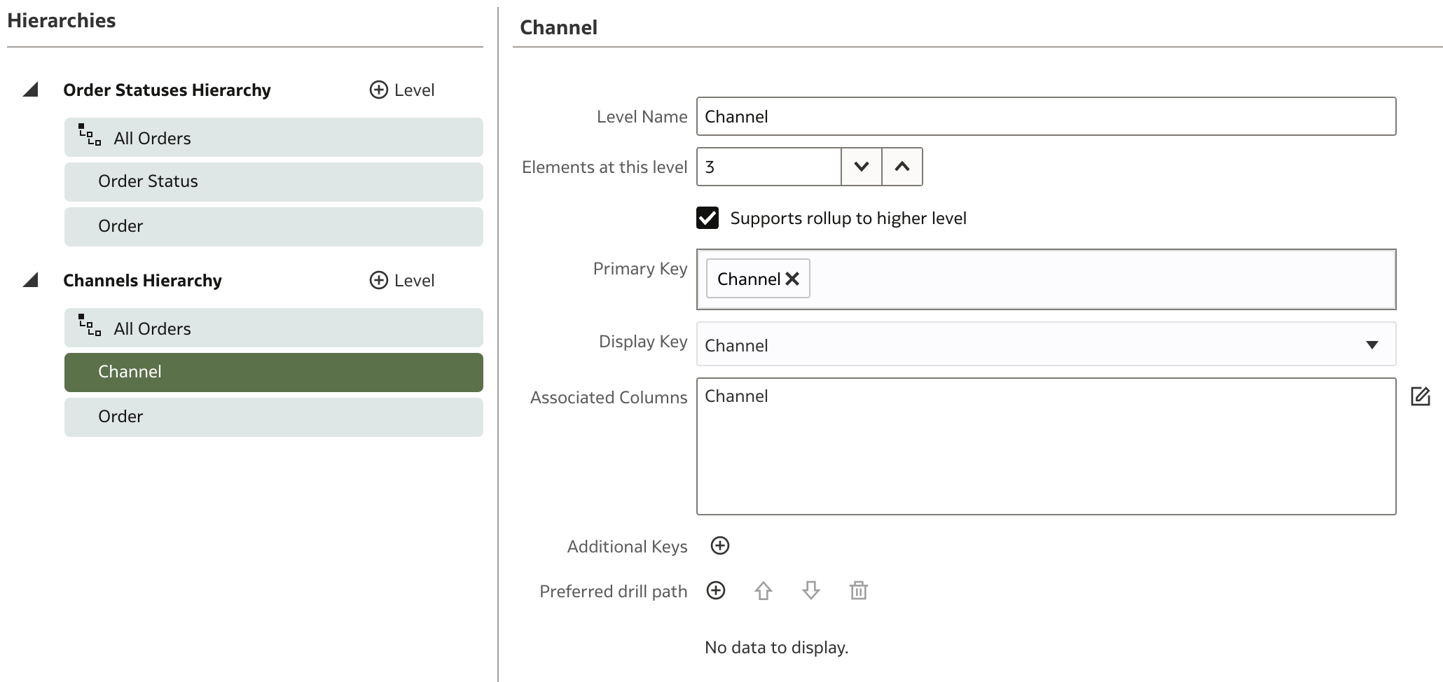
Similarly, you can define a second hierarchy for Channels:

Before moving on, let's create a join between the two tables defined so far: F Revenue and D Orders.

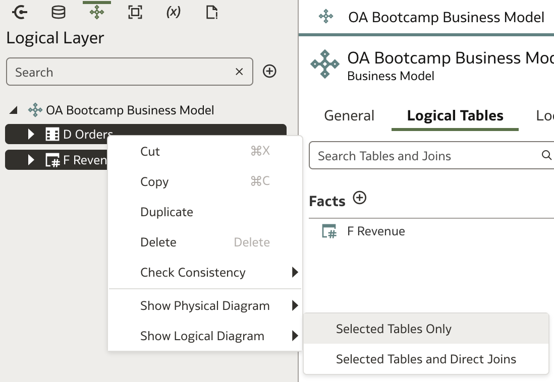
Expand the OA Bootcamp Business Model Logical Model in the navigation pane on the left.

Select both logical tables, right-click one, and select Show Logical Diagram. Expand it and choose Selected Tables Only.

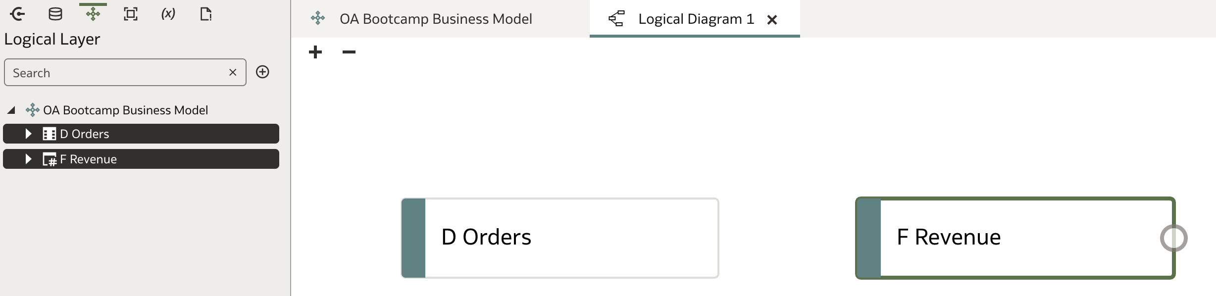
When the diagram appears, click the handle on one table (e.g., F Revenue) and drag the line onto the other (e.g., D Orders).

The Add Join dialog appears. In most cases, you can accept the defaults, but you may choose a different join type (e.g., Left Outer instead of Inner) or specify a Driving Table if required.

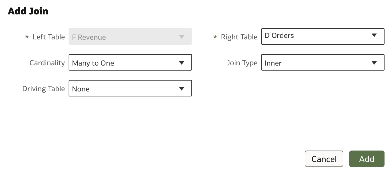
You have now successfully joined two logical tables. Note that no specific join conditions are required here—just the type of join—because join conditions were already defined in the Physical Layer.

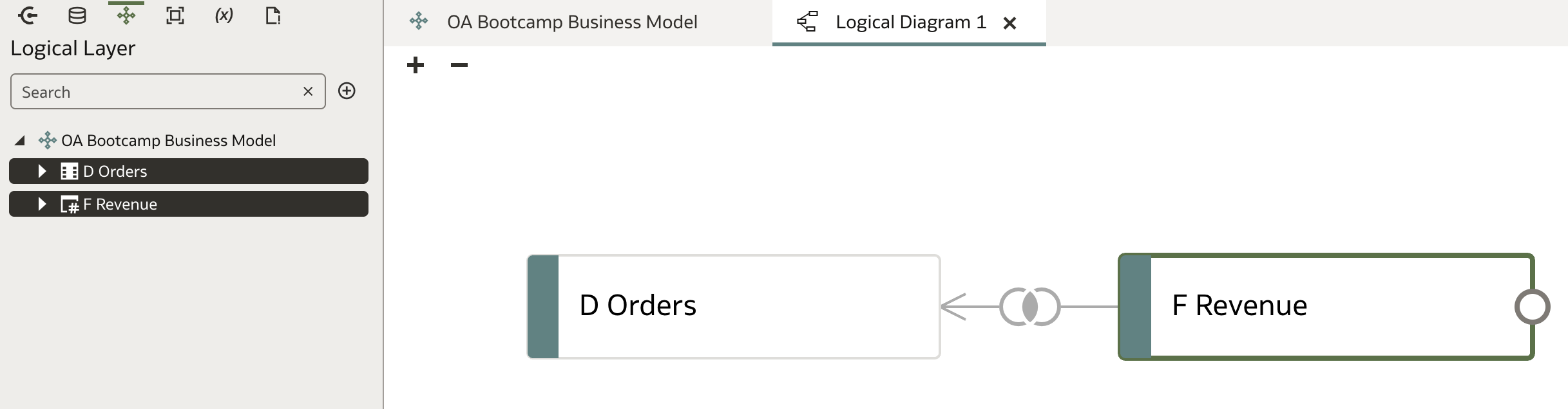
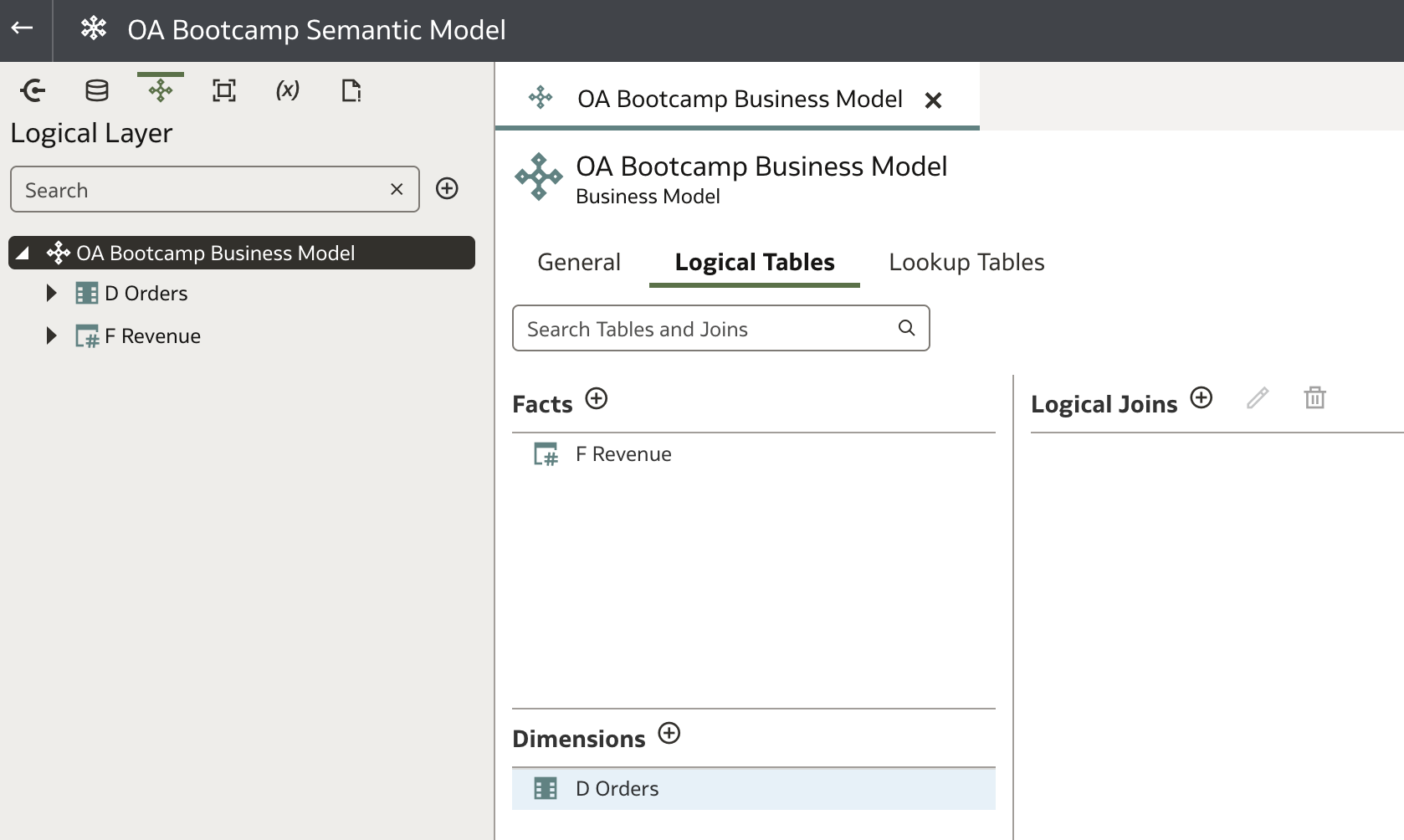
When you return to the logical model page, a new join should be displayed:

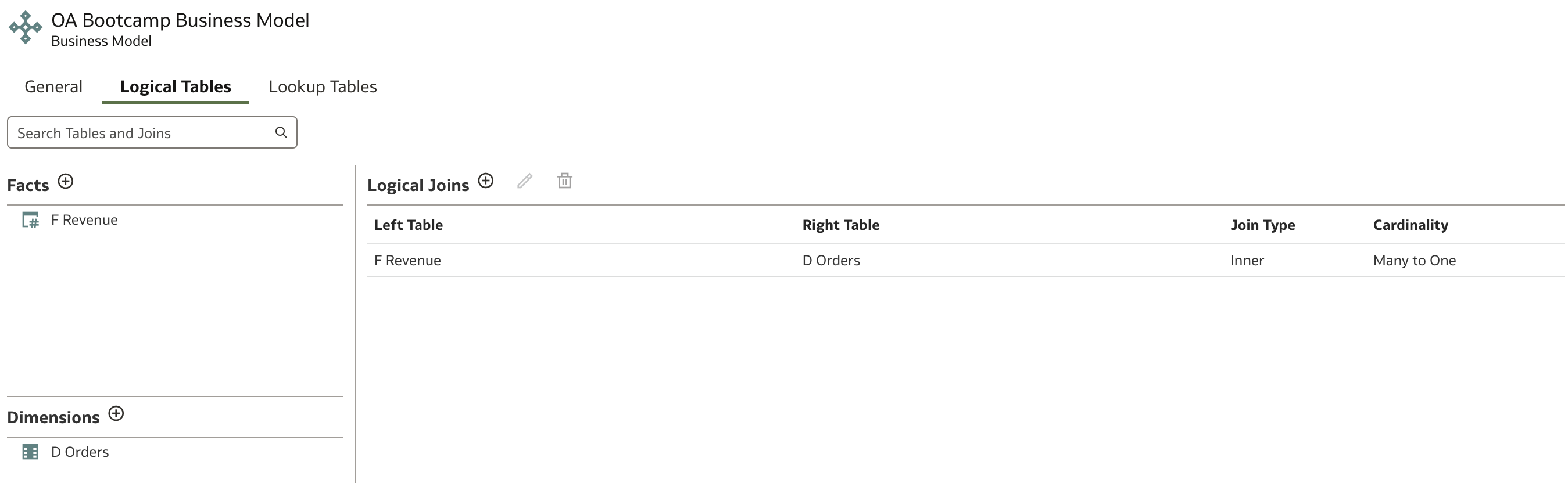
With this, you have defined your first dimension table and established a relationship with your fact table. There are still more dimensions to add. Close the D Orders page and return to OA Bootcamp Business Model.

Adding additional dimensions

Now, let's explore the drag-and-drop approach for importing physical tables into the logical model. Keep the OA Bootcamp Business Model page open. Then click Physical Layer to display all physical tables.

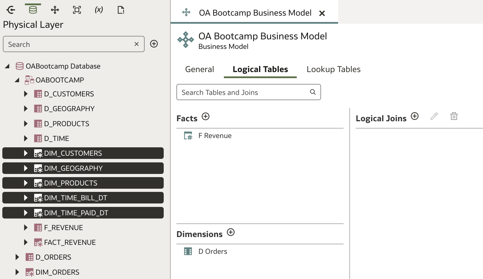
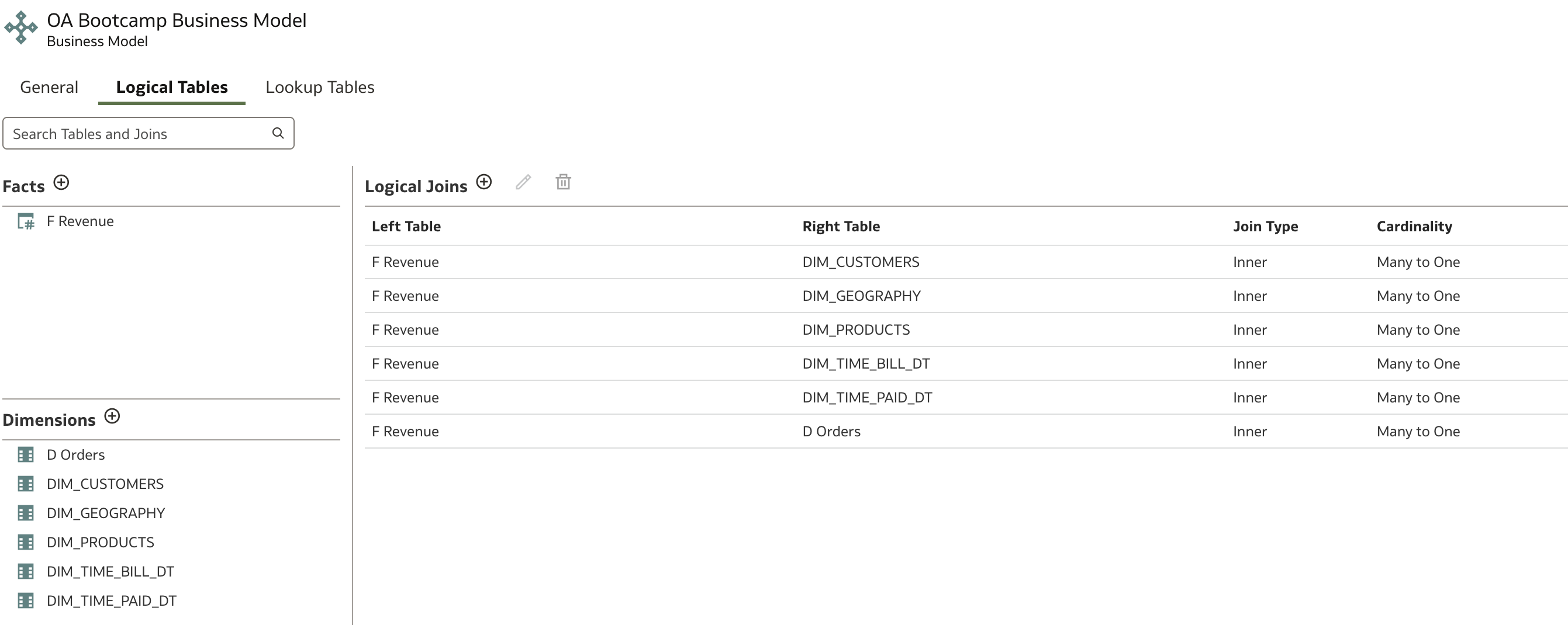
Drag all five dimension tables onto the Dimensions area of the OA Bootcamp Business Model page and drop them there.

Two things will happen:

• The selected dimension tables are added to the Dimensions list.
• Joins are also added based on definitions from the Physical Layer.

Now, make the dimensions user-friendly (e.g., rename columns) and add hierarchies where appropriate.

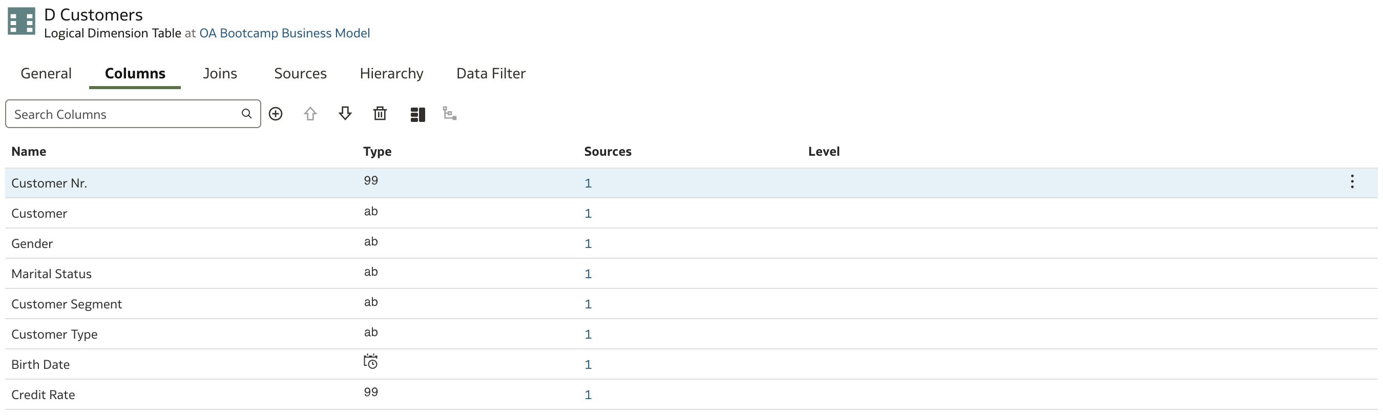
The dimensions DIM_CUSTOMERS, DIM_GEOGRAPHY, and DIM_PRODUCTS are straightforward, so let's review the final results:

D Customers dimension

D Geography dimension

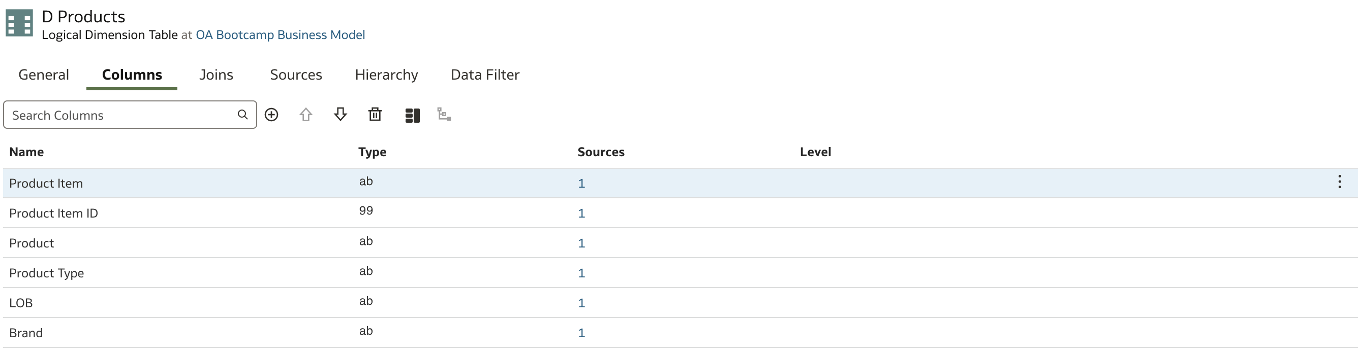
D Products dimension

Time Dimensions

There are two dimensions in our logical model that qualify as Time Dimensions.

Time dimensions are typically modeled as hierarchies (e.g., Year → Quarter → Month → Date). Defining hierarchies in this way enables users to drill down or roll up in visualizations and aggregate data at different levels.

In addition, marking a dimension as a Time Dimension allows developers to introduce a Chronological Key, which helps the BI Server understand the order of periods for time-series functions such as AGO, TODATE, or PERIODROLLING. These functions only work when a Time Dimension is properly configured.

Oracle Analytics supports the Gregorian calendar for time dimensions, but you can also implement additional calendars (such as fiscal calendars) if, for example, your fiscal year starts in July.

With Time Dimensions, you can create level-based measures (this applies to all dimensions). For example, Total Monthly Sales can be summarized at the Monthly level simply by specifying the correct aggregation level—no need for complicated formulas.

Whenever you define a dimension with date data, be sure to configure it as a Time Dimension; otherwise, it will behave as a regular dimension.

The two candidates for Time Dimension in our model are:

• DIM_TIME_BILL_DT
• DIM_TIME_PAID_DT

We'll define DIM_TIME_BILL_DT first, then repeat the process for DIM_TIME_PAID_DT.

Time Dimension: DIM_TIME_BILL_DT

Double-click DIM_TIME_BILL_DT in the Dimensions area of the OA Bootcamp Business Model page.

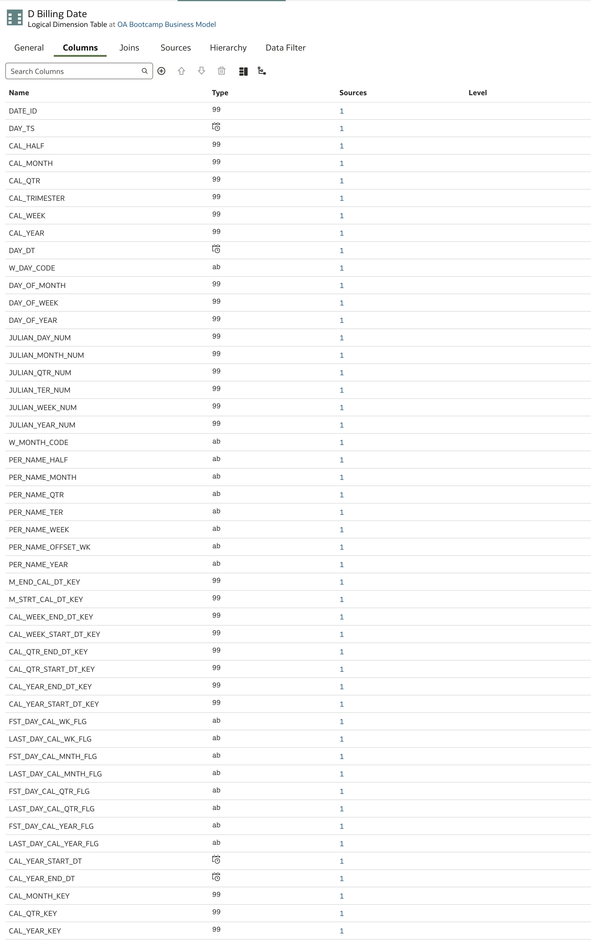
The DIM_TIME_BILL_DT page opens. You'll notice there are over 30 attributes, most of which are derived from the DAY_DT attribute.

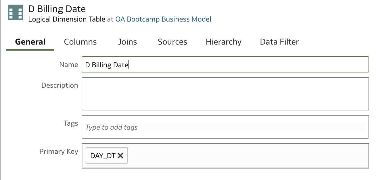
First, go to the General tab. Rename the dimension from DIM_TIME_BILL_DT to D Billing Date.

Next, go to the Columns tab. This step may take some time, but ensure that only the following columns are kept (delete all others):

• DAY_DT
• DAY_TS
• PER_NAME_WEEK
• PER_NAME_MONTH
• PER_NAME_QTR
• PER_NAME_YEAR
• DAY_OF_WEEK

You can delete columns one by one, but it may be faster to use the SMML Editor, which lets you update the definition as JSON-like code.

Save any changes made to D Billing Date so far. In the navigation pane, go to Logical Layer and click D Billing Date logical table.

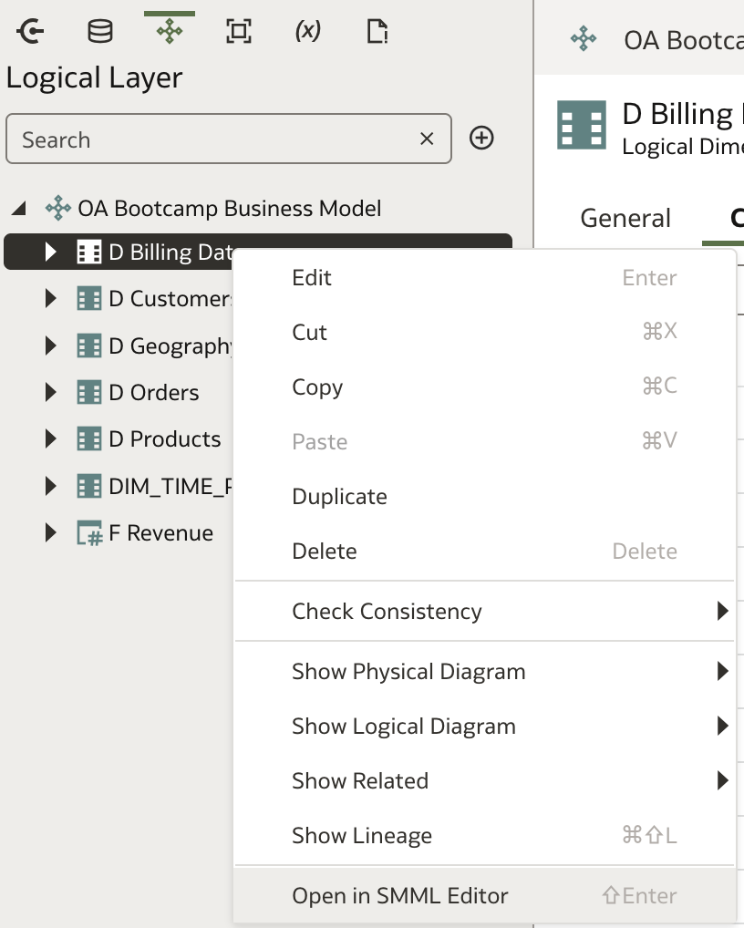
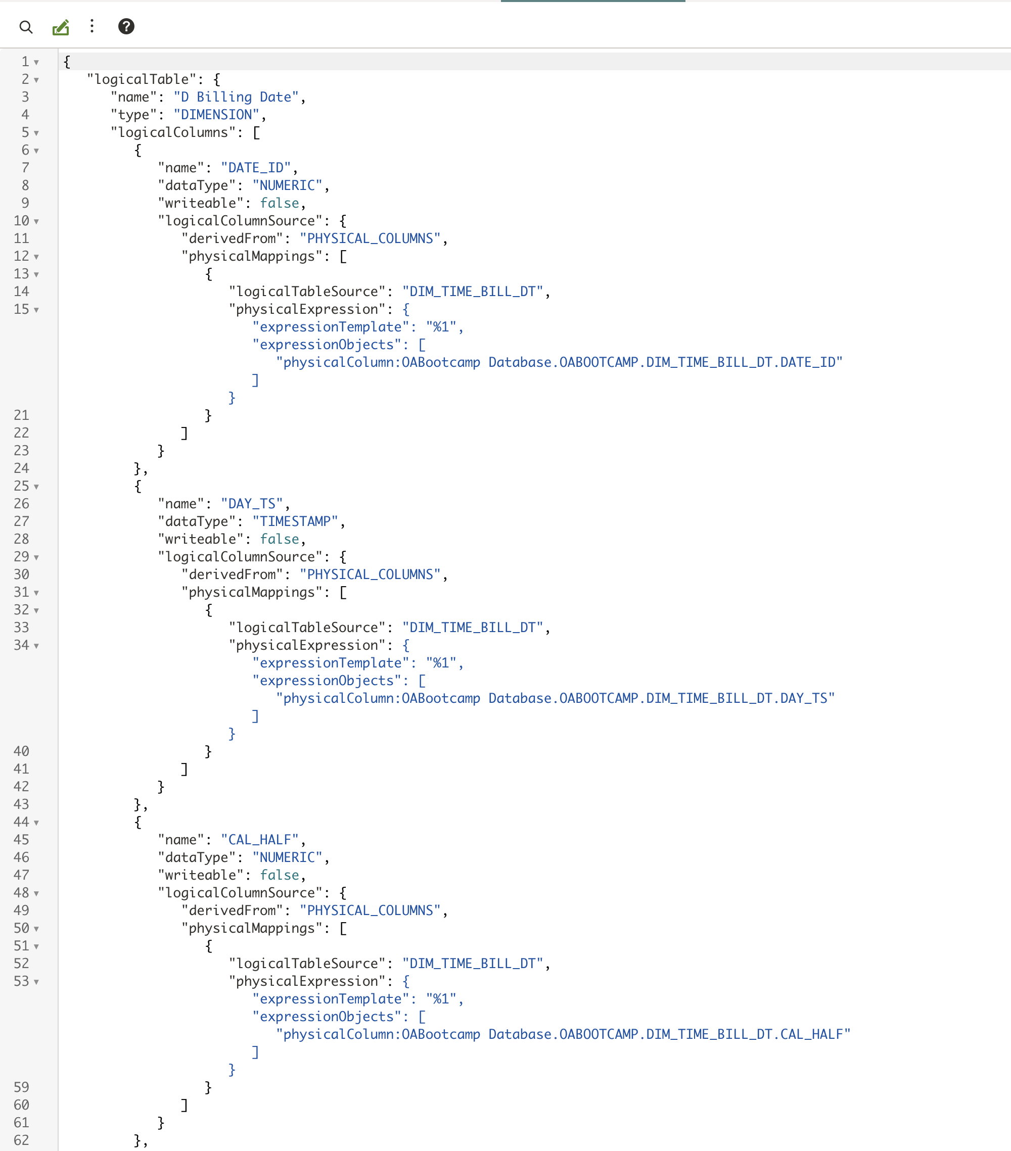
The SMML Editor opens with the column definitions. Each column is defined by a code block like this:

{
        "name": "DATE_ID",
        "dataType": "NUMERIC",
        "writeable": false,
        "logicalColumnSource": {
            "derivedFrom": "PHYSICAL_COLUMNS",
            "physicalMappings": [
                {
                    "logicalTableSource": "DIM_TIME_BILL_DT",
                    "physicalExpression": {
                    "expressionTemplate": "%1",
                    "expressionObjects": [
                        "physicalColumn:OABootcamp Database.OABOOTCAMP.DIM_TIME_BILL_DT.DATE_ID"
                    ]
                    }
                }
            ]
        }
    },
    

Remove the code blocks for all columns you don't need. This is a quick way to manage objects in the Semantic Model.

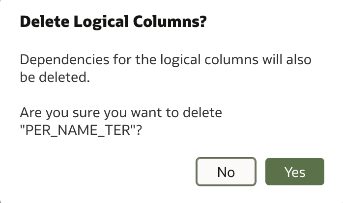
When you delete part of the code, a dialog appears to confirm your decision:

Once done, save your changes and close the SMML Editor.

Open the D Billing Date logical table page and check which columns remain. If you haven't already renamed columns in the SMML Editor, you can do it now.

Now, go to the Hierarchy tab. Since there are no hierarchies yet, select Time for Hierarchy Type.

The rest of the hierarchy definition follows the same process as before.

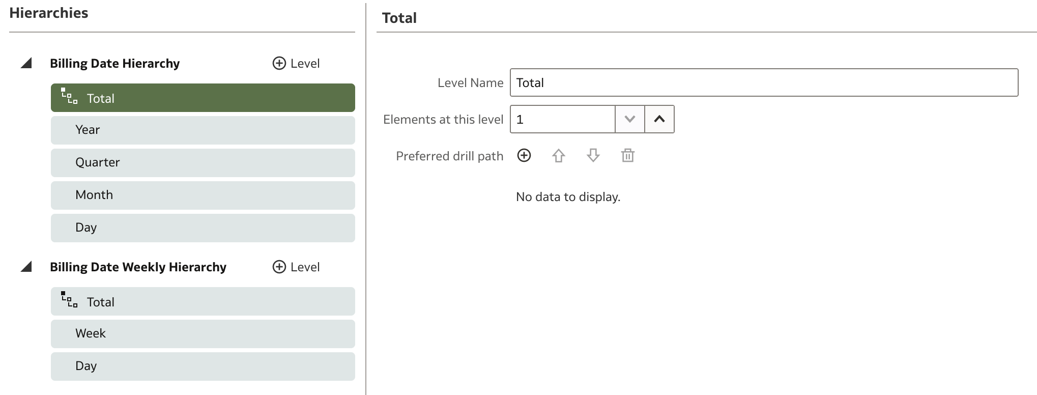
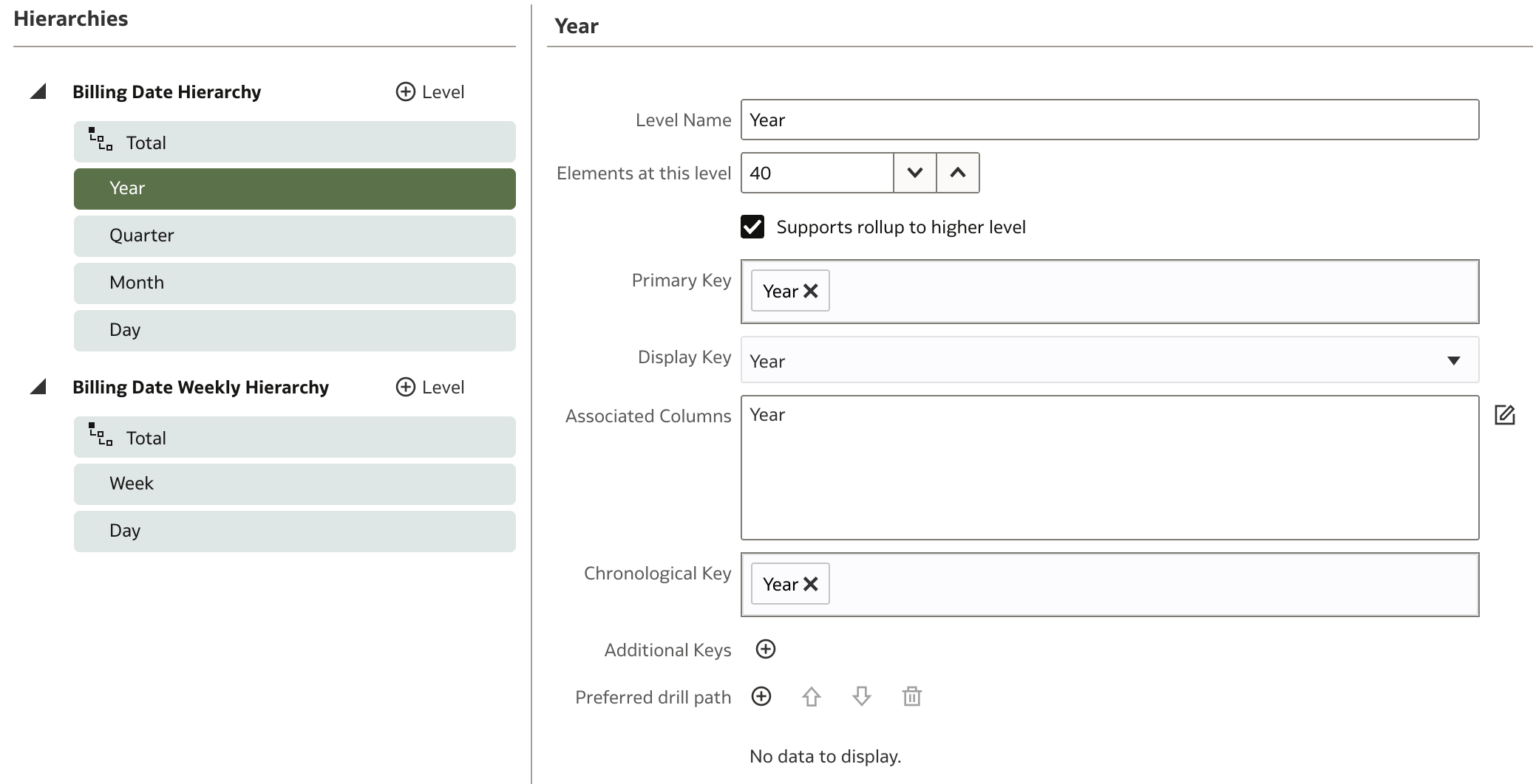
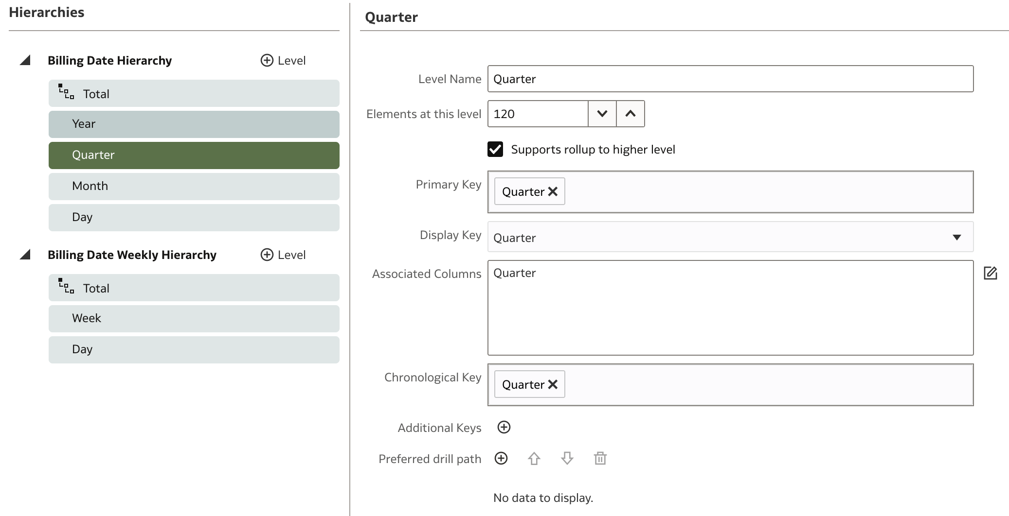
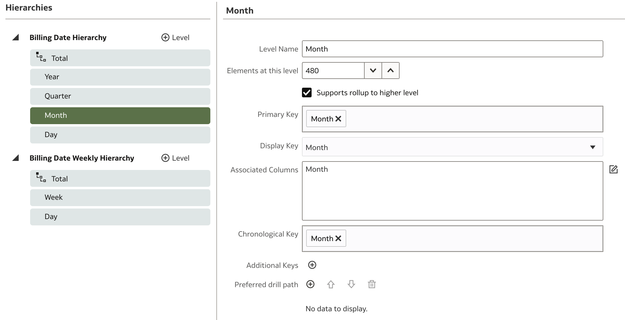
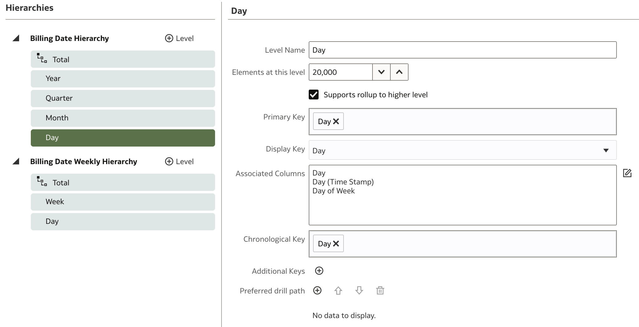
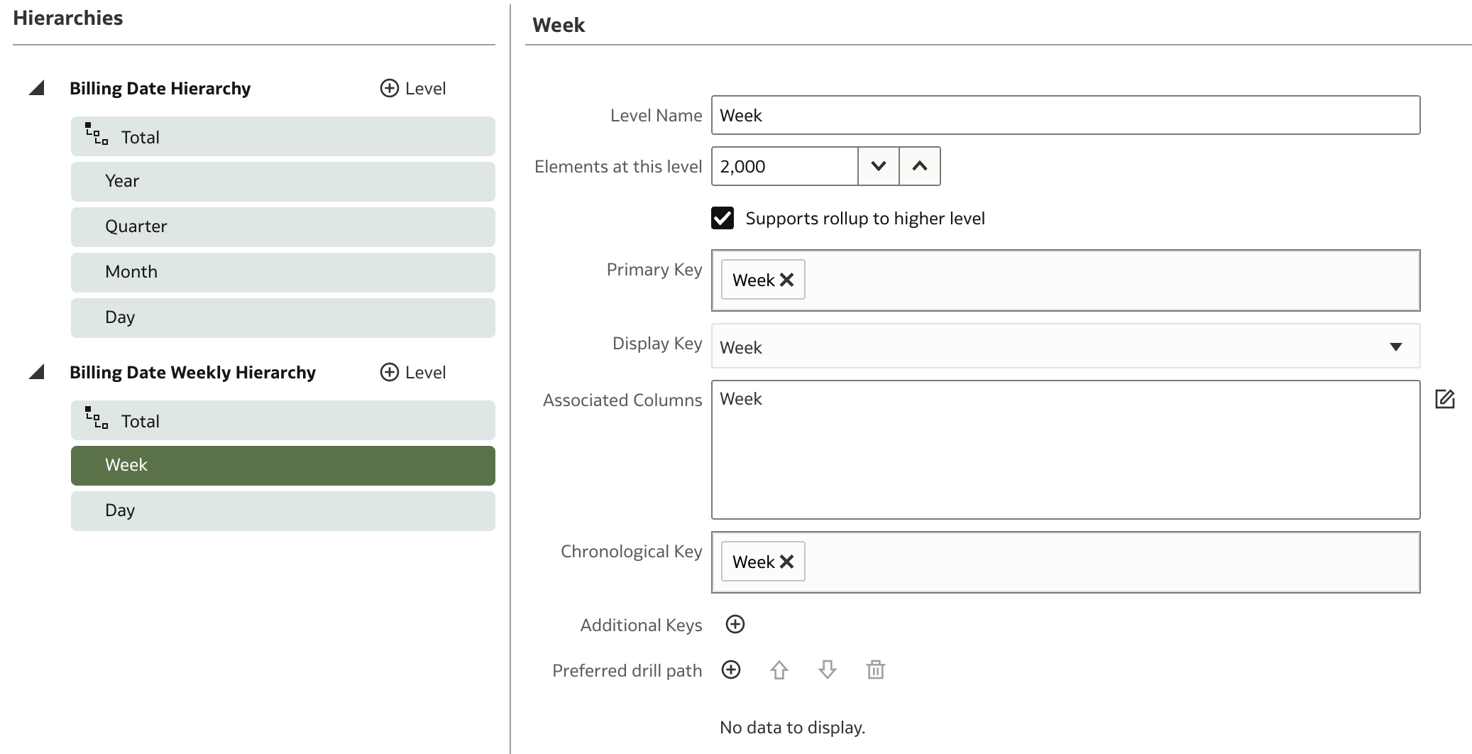
REMARK: Pay attention to the Chronological Key that is populated. Otherwise time series functions won't work properly.

Repeat the exact same steps for the other time dimension, DIM_TIME_PAID_DT.

Conclusion: Preparing for the Presentation Layer

In this session, we've explored the Logical Layer's critical role in Oracle Analytics. You learned how it abstracts and organizes physical data, defines logical tables and columns, establishes business relationships through logical joins, manages aggregations and calculations, and supports advanced scenarios such as hierarchies and time dimensions. By building a robust logical model, you've set the foundation for consistent, optimized, and user-friendly analytics.

With your logical model in place, you're now ready to move on to the next step: the Presentation Layer. The Presentation Layer will expose your business model to end users, allowing them to interact with the data in a secure, intuitive, and business-oriented way. Stay tuned for the next part of this series, where you'll learn how to prepare and publish your model for analysis!