Semantic Model Series 9: Data Fragmentation

What is Data Fragmentation

Data Fragmentation in Oracle Analytics refers to the practice of dividing large datasets into smaller, logically separated segments—called fragments—based on defined criteria such as time, region, or product category. This technique is primarily implemented in the semantic layer to optimize query performance and data management. By configuring fragmentation content filters on multiple logical table sources, Oracle Analytics can intelligently route queries to only the relevant data source, reducing processing time and improving efficiency. Fragmentation is especially useful in large-scale deployments where data is physically partitioned or spread across multiple tables or databases.

Just to clarify, when speaking of data fragmentation in Oracle Analytics, we’re not referring to table range partitioning, which is managed entirely at the database level and does not require any configuration in the semantic model, as partitioning is handled automatically by the database engine.

Let’s take a look at an example.

Import fragmented and mode data in Physical Layer

In the database, we have two tables that contain sales data for two different years: F_REVENUE_2022 and F_REVENUE_2023.

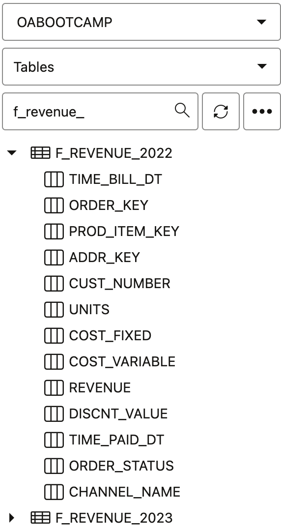
Both table have same structure, but can reside in different database (not in this case).

We need to import the metadata of both tables into the semantic model and properly link them to the dimensional tables—just as we would if there were only a single F_REVENUE table.

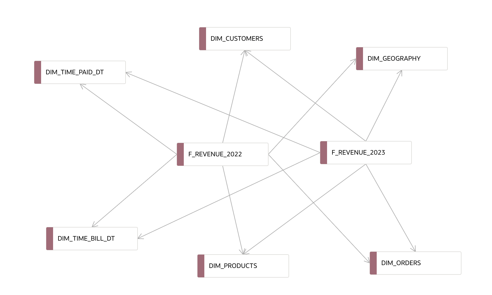
Following best practices, we also create aliases for these two tables to keep the model clean and maintain flexibility.

Once the aliases are in place, we can establish physical joins with all relevant dimension tables that relate to revenue, such as, in our case:

• DIM_TIME_BILL_DT
• DIM_TIME_PAID_DT
• DIM_PRODUCTS
• DIM_CUSTOMERS
• DIM_ORDERS
• DIM_GEOGRAPHY

Prepare Logical Layer

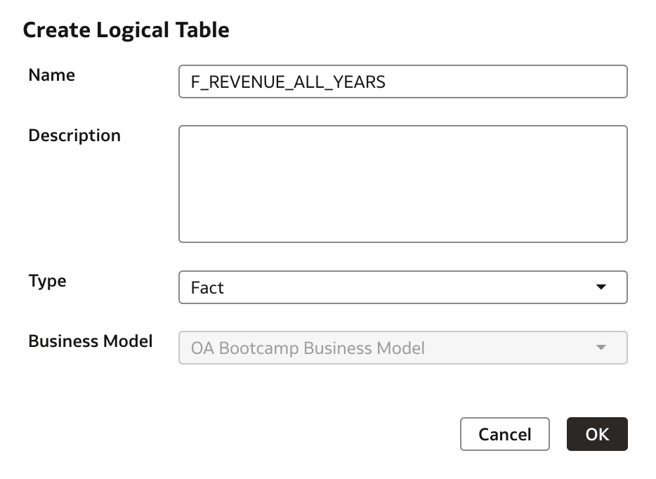
We can now continue setting up logical layer. First, we create a new logical table F_REVENUE_ALL_YEARS, for which we create 2 logical table sources.

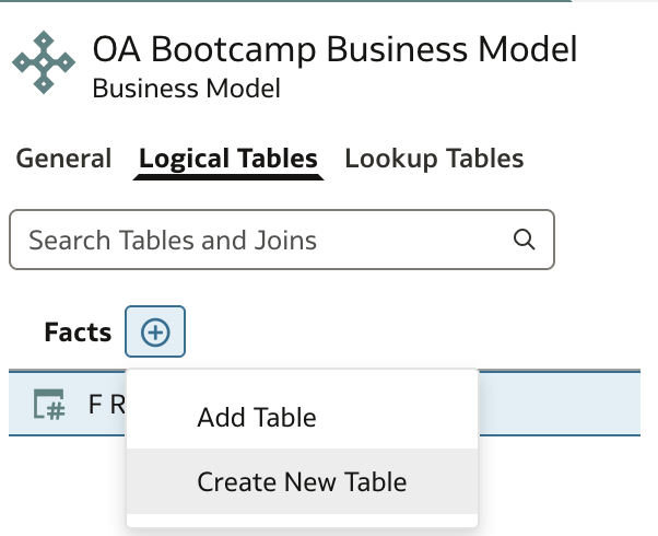
Provide a name for new logical table and continue:

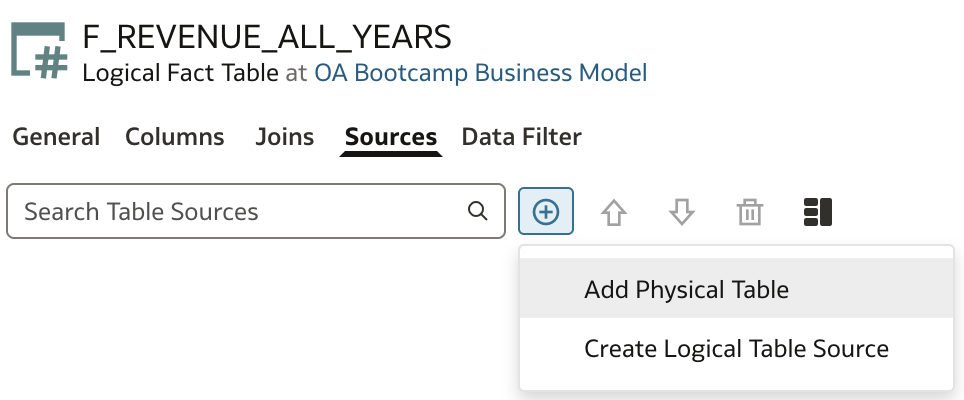
Once created, open new logical table in a separate tab and navigate to Sources tab and add both tables as logical table source:

Search for and mark both tables in Select Physical Table dialog:

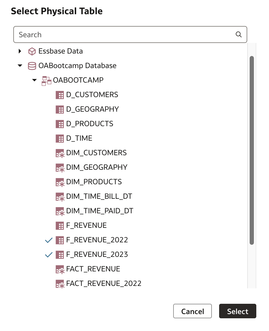
Click Select to continue.

Let’s check what we have at this point:

• Logical table F_REVENUE_ALL_YEARS has been created.

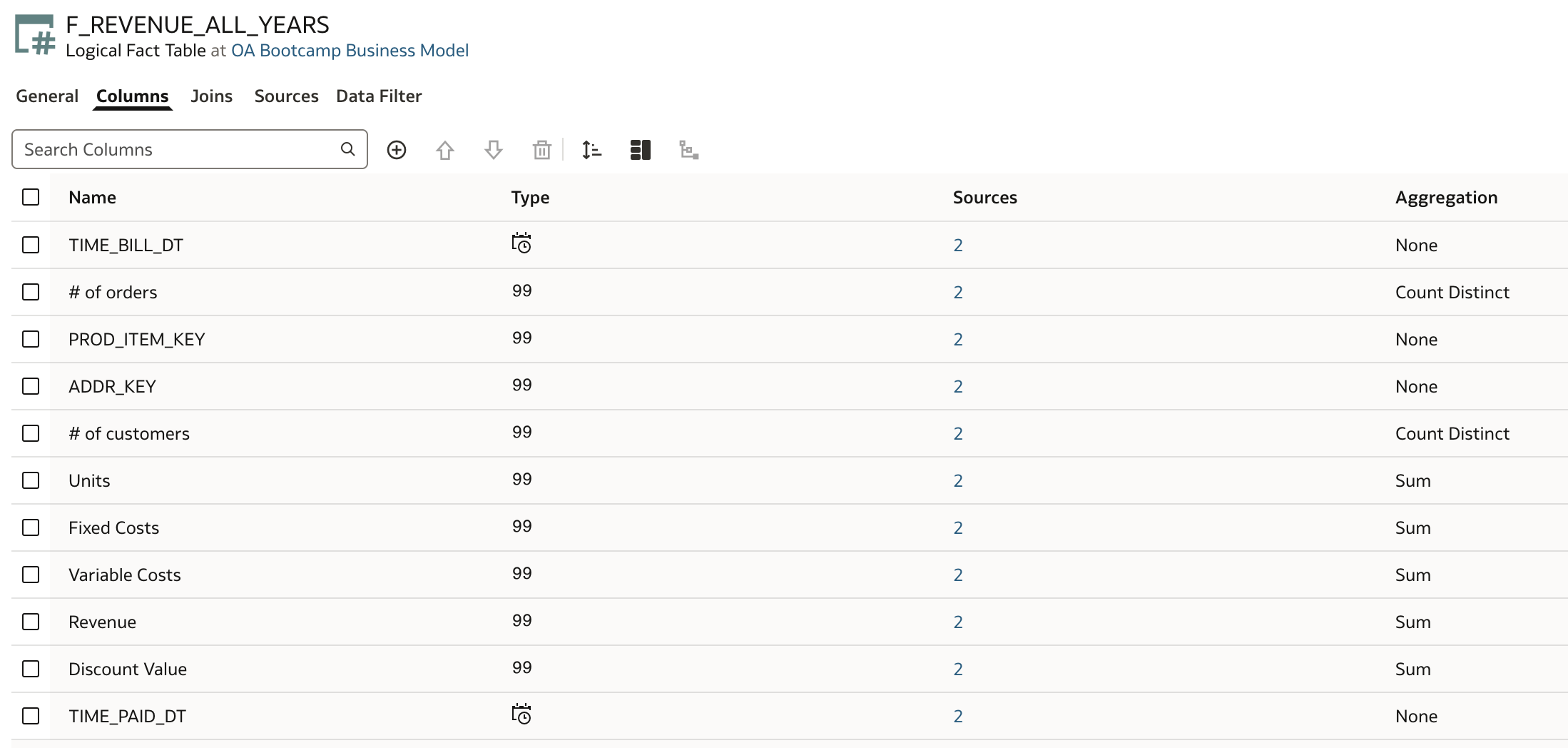
Before moving any further, make sure measures in this logical table are defined, not required attributes (ie- ORDER_STATUS) are removed ...

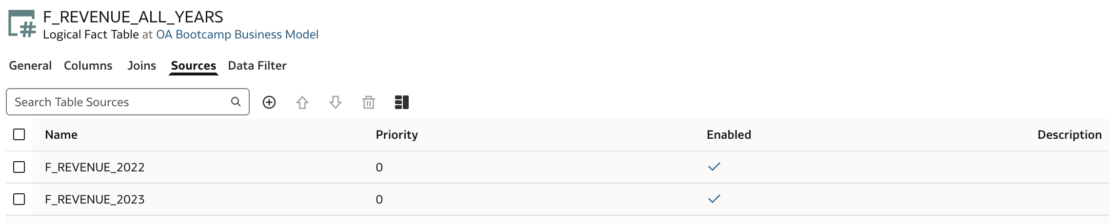
• F_REVENUE_ALL_YEARS has two logical tables sources.

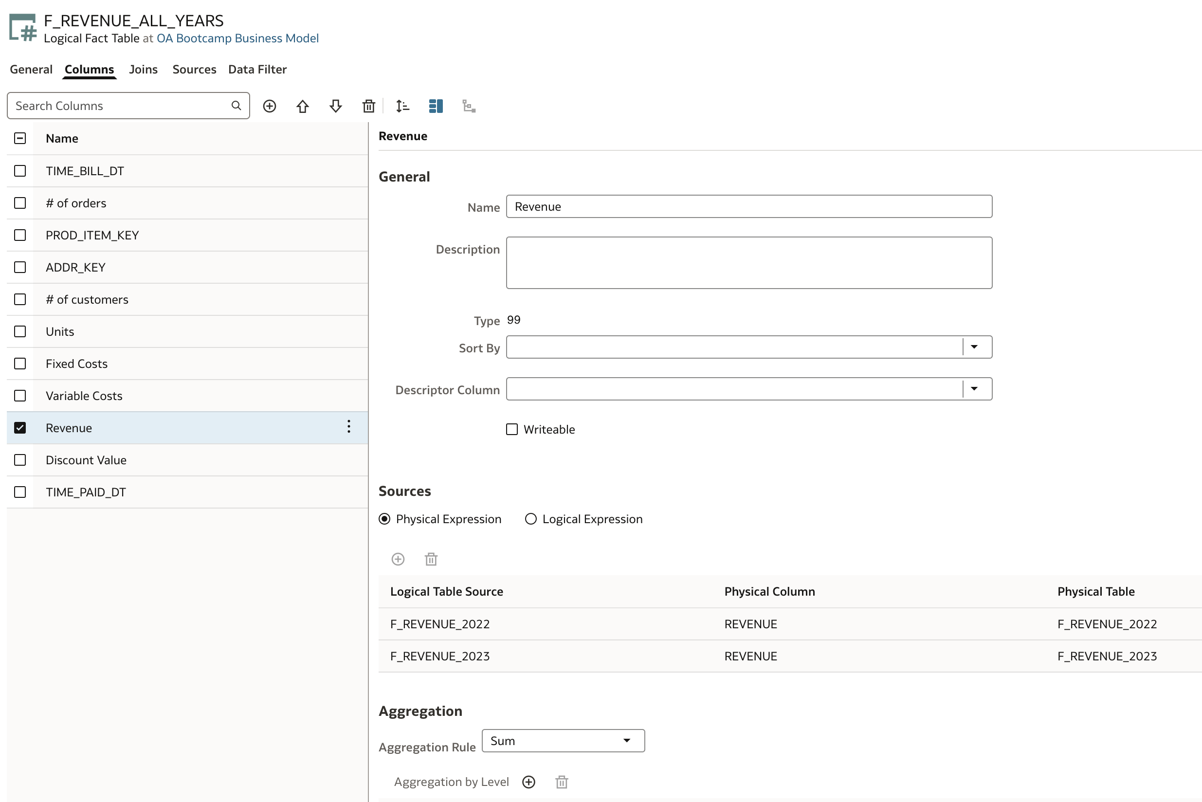
Let's drill to attribute level by opening detailed view for selected attribute, for example Revenue, in F_REVENUE_ALL_YEARS. We can observe that this attribute now has two Logical Table Sources: F_REVENUE_2022 and F_REVENUE_2023.

At this point, we are not ready for deploy, but let's check how the model would behave if we deployed it now. But before we deploy, there are a few more small tasks to take care of:

• We need to connect the tables in the logical model. The logical table F_REVENUE_ALL_YEARS was created manually, so the relationships from the physical model were not transferred automatically.

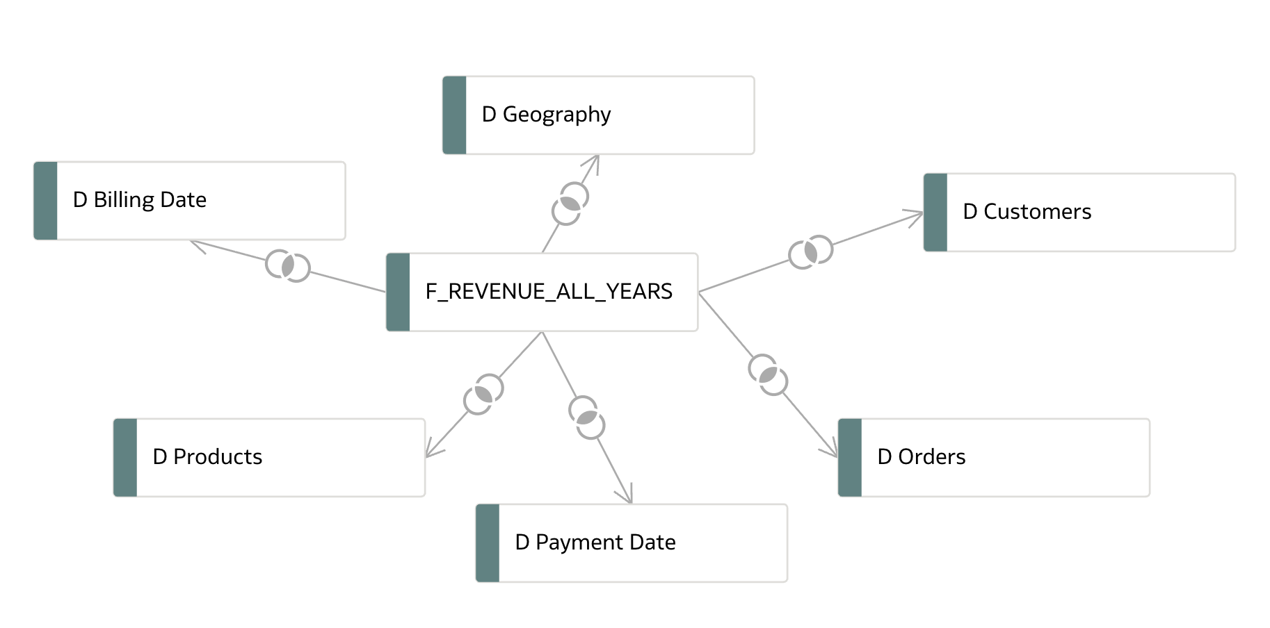
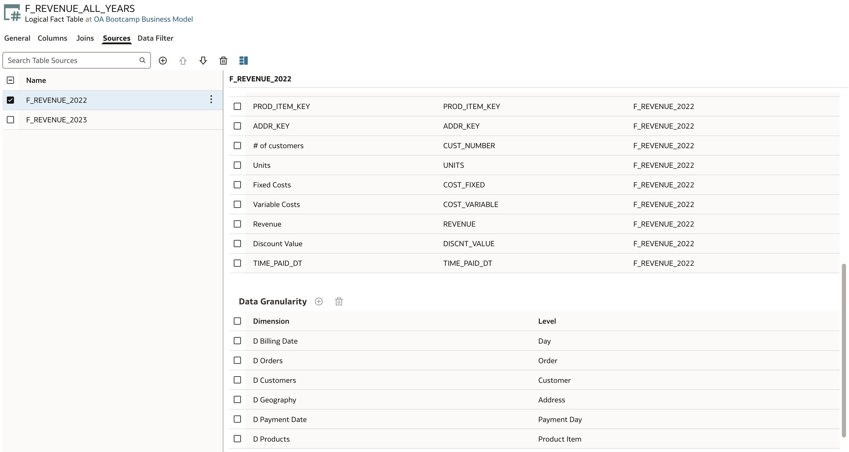
• Additionally, we need to define the correct levels by setting the appropriate levels of granularity.

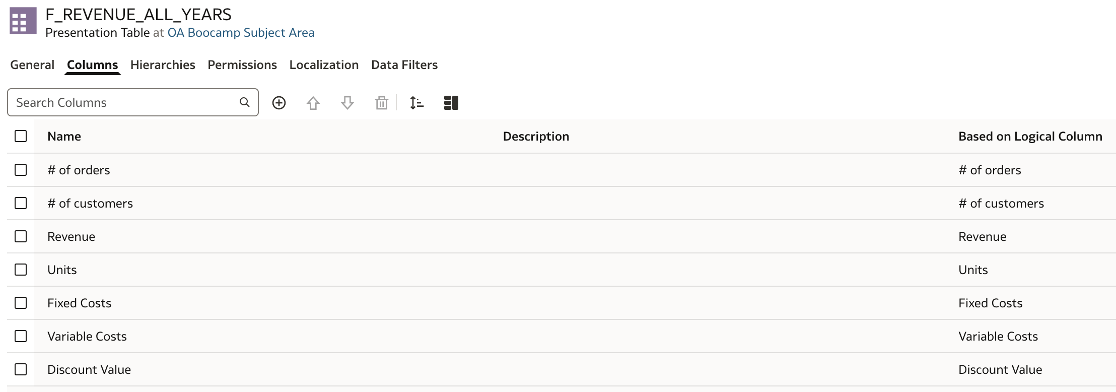
• Create a new presentation table in subject area.

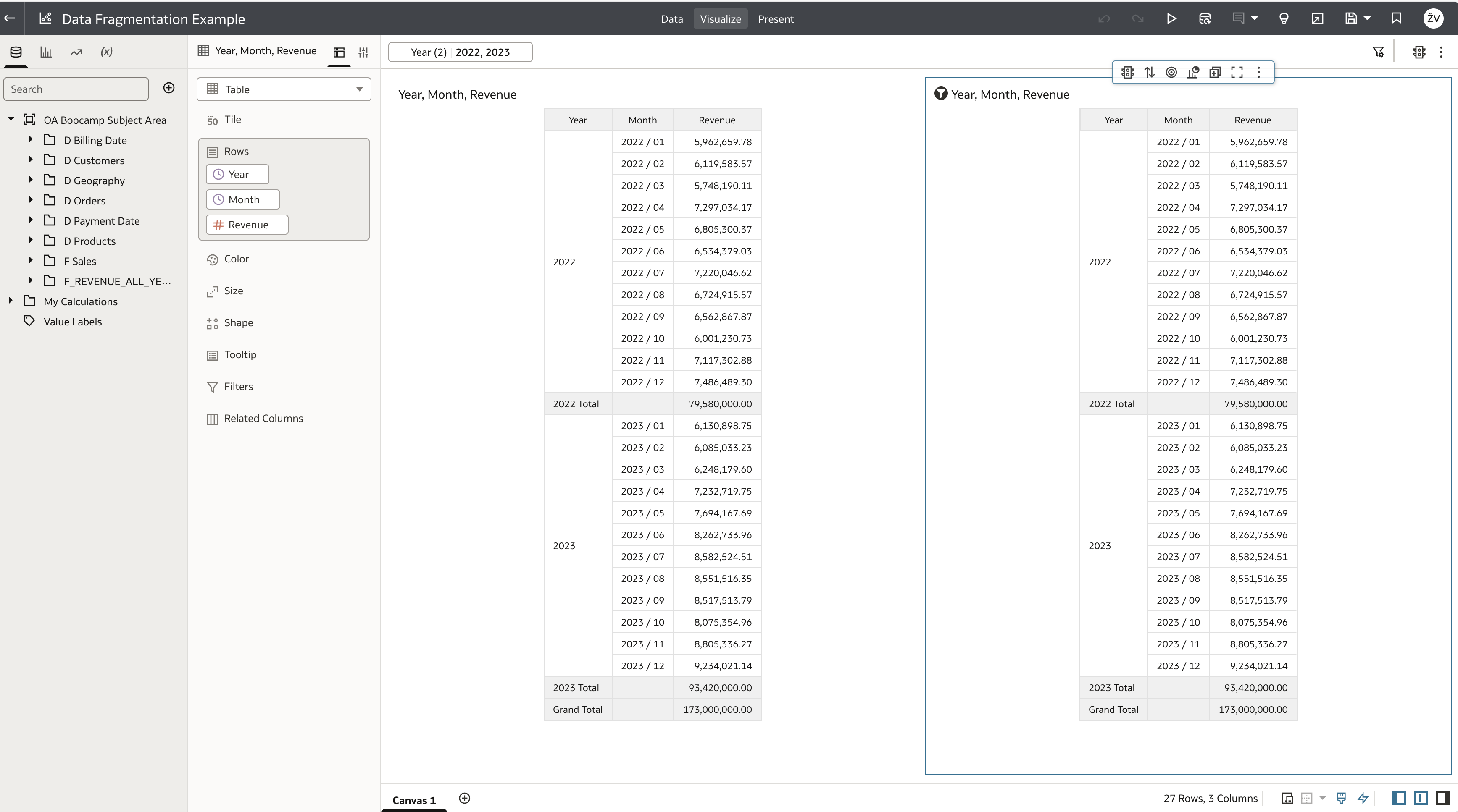
The workbook below displays what appears to be the same data in both tables. However, there's an important difference:

• The table on the left retrieves data from a single F_REVENUE table.
• The table on the right is reading only from the F_REVENUE_2022 table, which is defined as the first logical table source. As a result, no data is being retrieved from the second logical table source, F_REVENUE_2023.

This observation can be confirmed by reviewing script query generated by Oracle Analytics:

WITH 
SAWITH0 AS (
  SELECT 
    SUM(T114.REVENUE) AS c1,
    T19.PER_NAME_MONTH AS c2,
    T19.PER_NAME_YEAR AS c3
  FROM 
    OABOOTCAMP.D_TIME T19 /* DIM_TIME_BILL_DT */,
    OABOOTCAMP.F_REVENUE_2022 T114
  WHERE  
    T19.DAY_DT = T114.TIME_BILL_DT 
    AND T19.PER_NAME_YEAR IN ('2022', '2023')
  GROUP BY 
    T19.PER_NAME_MONTH, 
    T19.PER_NAME_YEAR
)
SELECT 
  0 AS c1,
  D1.c2 AS c2,
  D1.c3 AS c3,
  D1.c1 AS c4,
  0 AS c5,
  0 AS c6
FROM 
  SAWITH0 D1
ORDER BY 
  c3, c2;

There was no reference to the F_REVENUE_2023 table in the query, which is why no data for the year 2023 was retrieved.

How can we fix this? The answer is Data Fragmentation.

Configuring Data Fragmentation

Data Fragmentation is a simple step that is performed at each Logical Table Source where we specify data fragmentation condition.

Let's navigate to logical table sources. Under details for each of the source, we can find Data Fragmentation section.

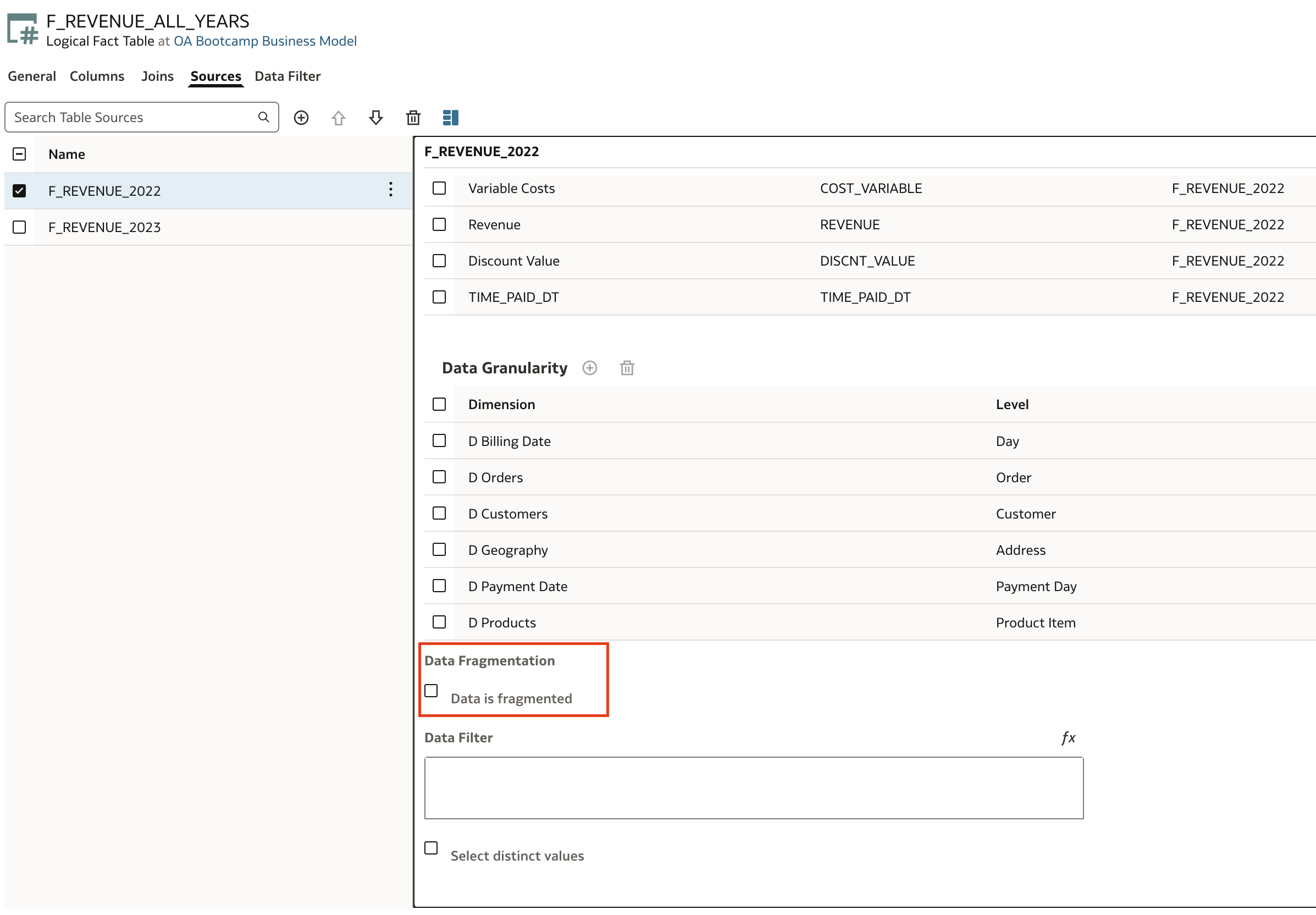
If data is fragmented as it is in our case, check Data is Fragmented check box. This will open addtional entry options.

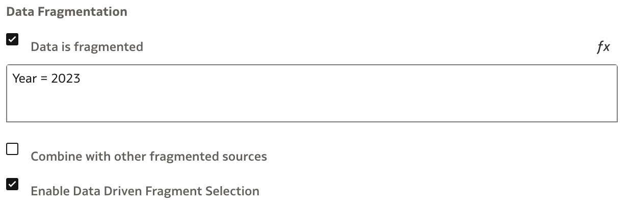
First, we need to define condition (aka filter) which tells BI Server which data is contained in this specific logical table source. For example, 2022 data.

Next, there are two additional parameters/options that we need to consider:

• Combine with Other Fragmented Sources
• Enable Data Driven Fragment Selection

Paremeter: Combine with Other Fragmented Sources

This setting tells BI Server that this logical table source (LTS) can be combined with other LTSs that also have fragmentation filters. For example, when we have multiple fragmented sources (e.g., one per year like F_REVENUE_2022, F_REVENUE_2023), enabling this allows the BI Server to union their results if needed — for example, when a report spans multiple years.

In our example, when we filter on:

WHERE "D Billing Date"."Year" IN ('2022', '2023')

Then both LTSs will be combined if this option is enabled. If it disabled, then only one LTS will be used in the query — which may lead to missing data or partial results.

Parameter: Enable Data Driven Fragment Selection

This setting allows the BI Server to dynamically determine which fragment(s) to query based on the actual data, even when no explicit filter (like "Year" = 2023) is provided by the user. This helps in scenarios where no year filter is applied in the report, or the year filter is coming from a prompt or a subquery. Oracle can inspect the data (via sampling or metadata) to determine which fragment to use — without a hardcoded filter.

If a user builds a report without filtering by year, and this option is enabled, then Oracle BI Server can still automatically include both LTSs and it is based on available data or context. If disabled, then BI Server may skip one or more LTSs unless an explicit filter matches a fragmentation predicate.

Let's examine what this actually mean in practice.

What is the difference?

Both data fragmentation filters are set for both Logical Table Sources and have Combine with Other Fragmented Sources checked.

We can run same report as before, and now also table on the right shows data from both logical table sources.

WITH 
SAWITH0 AS ((select T19.PER_NAME_MONTH as c2,
     T19.PER_NAME_YEAR as c3,
     T128.REVENUE as c4
from 
     OABOOTCAMP.D_TIME T19 /* DIM_TIME_BILL_DT */ ,
     OABOOTCAMP.F_REVENUE_2023 T128
where  ( T19.DAY_DT = T128.TIME_BILL_DT and (T19.PER_NAME_YEAR in ('2022', '2023')) ) 
union all
select T19.PER_NAME_MONTH as c2,
     T19.PER_NAME_YEAR as c3,
     T114.REVENUE as c4
from 
     OABOOTCAMP.D_TIME T19 /* DIM_TIME_BILL_DT */ ,
     OABOOTCAMP.F_REVENUE_2022 T114
where  ( T19.DAY_DT = T114.TIME_BILL_DT and (T19.PER_NAME_YEAR in ('2022', '2023')) ) )),
SAWITH1 AS (select sum(D3.c4) as c1,
     D3.c2 as c2,
     D3.c3 as c3
from 
     SAWITH0 D3
group by D3.c2, D3.c3)
select 0 as c1,
     D2.c2 as c2,
     D2.c3 as c3,
     D2.c1 as c4,
     0 as c5,
     0 as c6
from 
     SAWITH1 D2
order by c3, c2

As we can see, UNION ALL has been used to combine results from both logical table sources. For example, if we filter only on year 2023:

WITH 
SAWITH0 AS ((select T19.PER_NAME_MONTH as c2,
     T19.PER_NAME_YEAR as c3,
     T114.REVENUE as c4
from 
     OABOOTCAMP.D_TIME T19 /* DIM_TIME_BILL_DT */ ,
     OABOOTCAMP.F_REVENUE_2022 T114
where  ( T19.DAY_DT = T114.TIME_BILL_DT and T19.PER_NAME_YEAR = '2023' ) 
union all
select T19.PER_NAME_MONTH as c2,
     T19.PER_NAME_YEAR as c3,
     T128.REVENUE as c4
from 
     OABOOTCAMP.D_TIME T19 /* DIM_TIME_BILL_DT */ ,
     OABOOTCAMP.F_REVENUE_2023 T128
where  ( T19.DAY_DT = T128.TIME_BILL_DT and T19.PER_NAME_YEAR = '2023' ) )),
SAWITH1 AS (select sum(D3.c4) as c1,
     D3.c2 as c2,
     D3.c3 as c3
from 
     SAWITH0 D3
group by D3.c2, D3.c3)
select 0 as c1,
     D2.c2 as c2,
     D2.c3 as c3,
     D2.c1 as c4,
     0 as c5,
     0 as c6
from 
     SAWITH1 D2
order by c3, c2

We can see queries has been executed on both logical table sources using filter on year. The same results would be obtained even if no filter were used (e.g., if the filter were disabled).

WITH 
SAWITH0 AS ((select T19.PER_NAME_MONTH as c2,
     T19.PER_NAME_YEAR as c3,
     T128.REVENUE as c4
from 
     OABOOTCAMP.D_TIME T19 /* DIM_TIME_BILL_DT */ ,
     OABOOTCAMP.F_REVENUE_2023 T128
where  ( T19.DAY_DT = T128.TIME_BILL_DT ) 
union all
select T19.PER_NAME_MONTH as c2,
     T19.PER_NAME_YEAR as c3,
     T114.REVENUE as c4
from 
     OABOOTCAMP.D_TIME T19 /* DIM_TIME_BILL_DT */ ,
     OABOOTCAMP.F_REVENUE_2022 T114
where  ( T19.DAY_DT = T114.TIME_BILL_DT ) )),
SAWITH1 AS (select sum(D3.c4) as c1,
     D3.c2 as c2,
     D3.c3 as c3
from 
     SAWITH0 D3
group by D3.c2, D3.c3)
select 0 as c1,
     D2.c2 as c2,
     D2.c3 as c3,
     D2.c1 as c4,
     0 as c5,
     0 as c6
from 
     SAWITH1 D2
order by c3, c2

Let's now investigate the behaviour of the 2nd parameter, Enable Data Driven Frament Selection.

As we can see, Combine with Other Fragmented Sources and Enable Data Driven Frament Selection parameters are mutually exclusive, e.g. when selecting one, the other one is automatically deselected.

When testing the report above, and filtering only on 2023, table is properly filtered and underlying script is a follows:

WITH 
SAWITH0 AS (select sum(T128.REVENUE) as c1,
     T19.PER_NAME_MONTH as c2,
     T19.PER_NAME_YEAR as c3
from 
     OABOOTCAMP.D_TIME T19 /* DIM_TIME_BILL_DT */ ,
     OABOOTCAMP.F_REVENUE_2023 T128
where  ( T19.DAY_DT = T128.TIME_BILL_DT and T19.PER_NAME_YEAR = '2023' ) 
group by T19.PER_NAME_MONTH, T19.PER_NAME_YEAR)
select 0 as c1,
     D1.c2 as c2,
     D1.c3 as c3,
     D1.c1 as c4,
     0 as c5,
     0 as c6
from 
     SAWITH0 D1
order by c3, c2

We can see that only F_REVENUE_2023 was selected as a result of filtered data on 2023. This is definitely better than running a query with knowledge result of that subquery would be null. However, one must be carefull, as the following interesting thing happens when no specific filter is defined.

If we disable workbook filter, then the following happens:

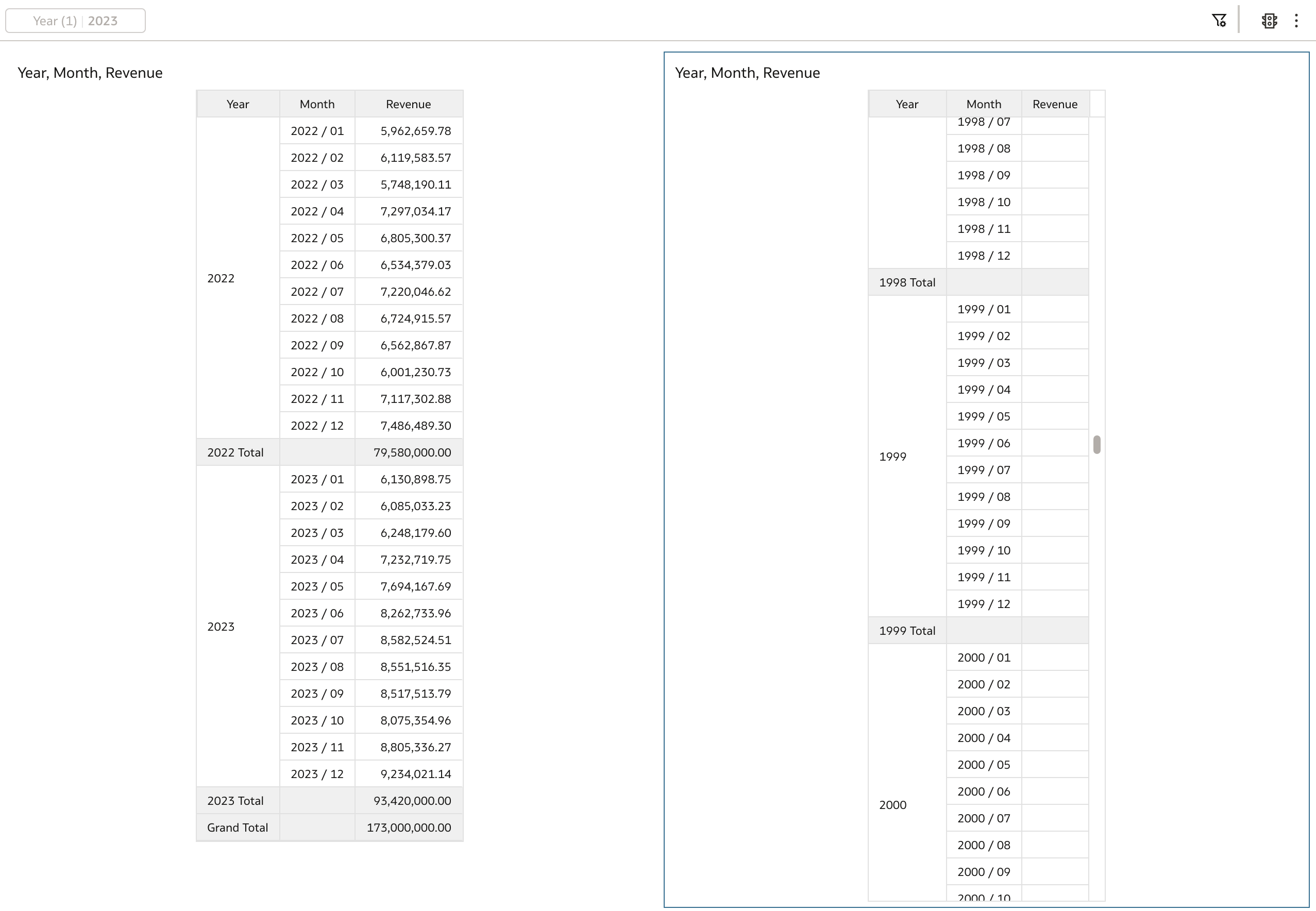
Only data from dimension table is displayed. Examining generated query shows that none of F_REVENUE_ tables were considered. This was kind of expected as logical table sourse selection is data driven and would only "pick up" logical table source when fragmentation condition is met. And in this particular case, none of conditions were met, hence no fact table at all in the query.

WITH 
SAWITH0 AS (select distinct T19.PER_NAME_MONTH as c1,
     T19.PER_NAME_YEAR as c2
from 
     OABOOTCAMP.D_TIME T19 /* DIM_TIME_BILL_DT */ )
select 0 as c1,
     D1.c1 as c2,
     D1.c2 as c3,
     cast(NULL as  NUMBER ( 38, 0 ) ) as c4,
     0 as c5,
     0 as c6
from 
     SAWITH0 D1
order by c3, c2

Conclusion

Data Fragmentation in Oracle Analytics is a semantic modeling technique used to optimize query performance by splitting large datasets into smaller, logically separate segments—called fragments. Each fragment is defined through a logical table source (LTS) with a content filter (e.g., for a specific year, region, or product group).

Oracle BI Server uses these filters to route queries only to relevant sources, reducing unnecessary data scans and improving performance.

Fragmentation is defined in the semantic model, not at the database level.

When working with data fragmentation, there are some best practices to follow:

• Define clear, non-overlapping filters for each fragment.
• Use Combine with Other Fragmented Sources for static, known splits (e.g., per year).
• Use Data Driven Fragment Selection when the filter is optional or dynamic.
• Avoid overlapping fragmentation filters to prevent data duplication or loss.
• Monitor query logs and test behavior without filters to verify LTS selection.
• Use alongside aggregate persistence or summary tables for larger datasets.