
Oracle Data Lakehouse Series highlights some of the examples of using elements of Oracle Data Lakehouse and presents the tools that are available as part of Oracle Cloud Infrastructure.
The first blog, Using OCI Object Storage based Raw Data in Oracle Analytics, of the Series talks about how to use Object Storage for “a file cabinet” for the retail transactions CSV files. These files are then “registered” with Oracle autonomous database and used in Oracle Analytics analyses. Any new files added to that “file cabinet” are immediately included in any analysis.
Of course, there are several ways to perform the following exercise, but in this 2nd example I’m discussing similar approach to load and use the data, however there are two add-ins in the process. Firstly, we will use Oracle Analytics Data Flows to prepare data for machine learning exercise and secondly we will use Oracle Machine Learning AutoML feature to build a prediction model which will be registered with and used in Oracle Analytics.
This time, we are using Kaggle’s Telecom Churn Case Study Hackathlon dataset.
Data ingestion


Preprocessing data
In this step of the process, data is made accessible from Oracle Database and transformations are applied by using Oracle Analytics Data Flows.
Creating an external table
Procedure to create an external table is the same as described in my previous blog. The only difference is that this time we need to create two external table, one of training (churntrain.csv) and one for new data (churntest.csv). In my previous example, we referred to all CSV files in a folder.The script to create an external table could look like this (there are 100+ columns in the CSV file which should have been listed in the right order):
DBMS_CLOUD.CREATE_EXTERNAL_TABLE(
table_name => 'CHURN_TRAIN',
file_uri_list => 'https://objectstorage.eu-frankfurt-1.oraclecloud.com/n/<bucket_namespace>/b/telecom-churn-data/o/churntrain.csv',
format => json_object('type' value 'csv', 'skipheaders' value '1', 'delimiter' value ',', 'rejectlimit' value '100'),
column_list => 'ID NUMBER,
CIRCLE_ID NUMBER,
...
CHURN_PROBABILITY NUMBER’
END;
/
Parameter file_uri_list points to file location in a bucket list. Careful reader might spot that there is no credential_name parameter in the CREATE_EXTERNAL_TABLE call. This is not required as we are using Pre-Authenticated Request.
Using OAC Data Flows for data preprocessing and preparation
Data Flows are very useful and convenient, self-service, data preparation and augmentation tool that is part of Oracle Analytics. We could have used different tools to do the same thing here, but the idea is to use Data Flows to make some data preparation activities and store data into database at the end.
As I said, same steps could easily be achieved by making transformation using SQL or Python or any other ETL tool.
Working with datasets in Oracle Analytics is really user friendly and any end user could learn it pretty fast.
It all starts with a new dataset that is based on a database table or even SQL query. In its simplest form is just drag & drop exercise.

The tool automatically performs dataset profiling, hence trains itself to present the user with recommended transformations in order to enrich current data.
In our example, we will use Convert to Date function, which converts text dates into proper Date Format. We could perform most of transformations here, however, I found it a bit easier to use a Data Flow. And since there are two datasets that require exactly same transformations, I decided to to most of the transformations using Data Flows.
The Data Flow consist of several steps which are quite intuitive and enable user to perform necessary changes. For example, several columns contain only one value, or date columns are either one or a lot of values. That is why additional columns are created, such as Day of Week and Day of Month for all Date columns. Finally, a new, clean dataset is stored.

To apply the same Data Flow on the New dataset (the one used in prediction), only the right database table has to be selected in the first step. All other steps are unchanged from the original Data Flow which prepares data for model training.
So, after both data flows or sequence (we could create a sequence which execute both data flows one after another) is completed, we end up with two new database tables CHURN_TRAIN_CLEAN and CHURN_TEST_CLEAN.
We will use these two tables in the next steps. If data was clean already at the beginning, then we would perform all of the following steps using original CSV files stored in object storage.
Predict & Analyze
In this process step, I will apply AutoML to train and predict churn, and consequently the results, the best model, will be registered and used with Oracle Analytics.
Using AutoML UI
Oracle defines AutoML User Interface (AutoML UI) “as an Oracle Machine Learning interface that provides users no-code automated machine learning. Business users without extensive data science background can use AutoML UI to create and deploy machine learning models.” .

We will use AutoML UI to train several machine learning model and identify the most appropriate for the predicting churn on the set of new data.
As definition itself says, the process of using AutoML UI is code-less. Users need to provide some basic information about their data and set some settings in order to start the process which automatically and autonomously undertakes the following activities:
- algorithm selection,
- adaptive sampling,
- feature selection and
- hyperparameter tuning.
All of these steps are usually done by developer, and here we see the whole process automated.
Each AutoML process is called experiment. User is required to set some basic parameters, like name and comments.
Data source, a database table, is selected from the list of available database tables. Once Predict (target column) and Case ID are selected, Prediction Type is automatically detected.

Additional Settings are already pre-populated, but one can adjust to his needs. Users can run and optimise a model training by selecting one of the standard Model metrics such as Accuracy, Precision, Recall, ROC AUC and others.


Just a remark, this is obviously linked to the duration parameter set in Additional settings. If this is not set adequately, one might get better results if Faster Results is selected.
AutoML then runs itself. Pop-up window Running is displayed and progress can be tracked alongside graphical presentation of the current best Model metric.

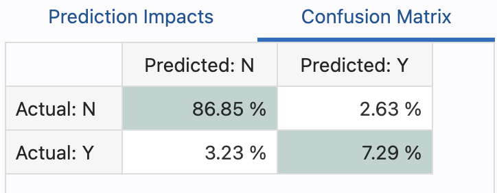
After the process is completed, algorithms are sorted by the value of observed metric. More details are available, such as which columns impact the prediction the most:

or you can observe the confustion matrix:

Registering and using the best ML model with Oracle Analytics
In the last section of this blog post, let’s focus on how to use the model we created using AutoML UI. One way of using it could be Oracle Analytics. So let’s take a look how this can be done.
First, the model created just earlier needs to be registered with Oracle Analytics. As you can see all information related to a model is accessible before model is registered.

When model is successfully registered, it can be used in Data Flows. Apply Model step applies machine learning model on the dataset selected. In this case, this is new clean data which requires Churn prediction.

The output of the step will be two new columns, Prediction and Prediction Probability.

At the end, Data Flow stores a new dataset with predictions to the database or to dataset storage. Now, the “prediction” dataset can be used in a workbook and visualised.

Conclusion
This blog post discusses one possible approach how to use predictive analytics in Oracle Data Lakehouse alongside Oracle Machine Learning and Oracle Analytics. This is definitely the only alternative and maybe dataset selected is potentially not the best example. However, I think that the discussion above highlights possibilities one might have using Oracle Data Lakehouse platform.
In the next blog in this series, we will take a look at the other side of the Data Lakehouse and explore how we could capture and process Streaming data.