In my previous post, I have described how "out-of-the-box" analytical functions in Oracle Data Visualisation Desktop or Oracle Data Visualisation Cloud Service could be used very easily and efficiently.
In this blog, we will explore how to create new measures using standard analytical functions that are available in Formula Builder.
Like "out-of-the-box", you can use the following analytical functions:
- Trendline: Fits a linear or exponential model and returns the fitted values or model. The numeric expr represents the Y value for the trend and the series (time columns) represent the X value.
- Cluster: Collects a set of records into groups based on one or more input expressions using K-Means or Hierarchical Clustering.
- Outlier: This function classifies a record as Outlier based on one or more input expressions using K-Means or Hierarchical Clustering or Multi-Variate Outlier detection Algorithms.
- Regr: Fits a linear model and returns the fitted values or model. This function can be used to fit a linear curve on two measures.
- Evaluate_Script: Executes an R script as specified in the script_file_path, passing in one or more columns or literal expressions as input. The output of the function is determined by the output_column_name. We will discuss this function call in my final post of the series.
Even though Forecast is listed in Time Series functions, it can be considered as a Analytical function and that is why I am presenting it in this post.
Add a New Calculation
Let's take a look how can one add a new calculation. Open Data Visualisation Desktop (all steps are the same for DVCS as well).
Open Data Elements panel and locate Add Calculation link at bottom right corner of the panel (not canvas). Click on it.

Obviously, new calculation has to be named, but on the right panel, you can scroll down to Analytics functions and expand the subtree to check for available functions. All five functions are displayed.
You can click on one function and its syntax will appear in the formula box on the left.
Trendline
Let's create a line chart visualisation with Order date as a Category and Customer Segment (filter on value Customer) and Gross Unit Price as a measure:

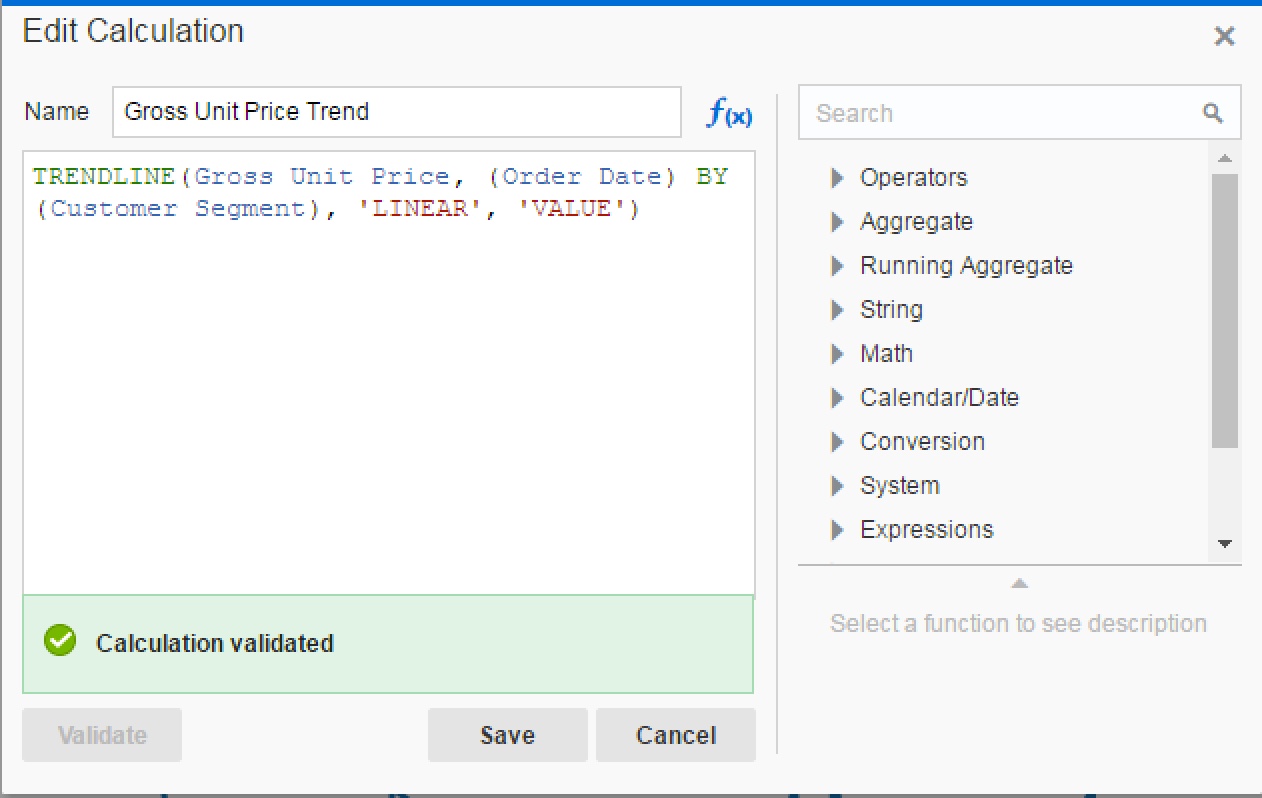
If you want to create a new calculation using Trendline analytical function use the following syntax:
TRENDLINE(numeric_expr, ([series]) BY ([partitionBy]), model_type, result_type)
numeric_expr is plotted on Y axis and is a measure in most cases, for example Sales or Gross Unit Price in our case. series is in most cases a time series attribute, in our case Order Date and it is plotted on X axis. partitionBy is an attribute or attributes that is included in the view but not displayed on X axis. model_type can be LINEAR or EXPONENTIAL and result_type is VALUE or MODEL. VALUE returns regression values for given X values in the sample. MODEL returns all parameters.
Create a new calculation now:
And add calculation to the chart:

The light blue line shows the linear trend. You could have selected EXPONENTIAL instead of LINEAR. Example below shows both Trend lines, exponential is the lower one.

Since Trend is now a measure, it can be used to create new additional calculations. This is not possible with "out-of-the-box" analytical function which were discussed in my previous post. For example, let's assume that difference between Linear and Exponential trend might be interesting to someone:

Cluster
The second analytical function is Cluster. We have seen how easy is to apply "out-of-the box" clusters in the graph. Similarly that is just a visualisation. With Cluster analytical function, a new calculation is created in the data set.
Let's begin with the following visualisation:

Cluster function has the following syntax:
CLUSTER((dimension_expr1 , ... dimension_exprN), (expr1, ... exprN), output_column_name, options, [runtime_binded_options])
dimension_exprN are dimension attributes which will be used for clustering. exprN are attributes that will be used to ctuster dimension_exprN attributes.
There are several options for output_column_name. You can choose among the following: clusterId, clusterName, clusterDescription, clusterSize, distanceFromCenter and center.
In the picture below you can check the results of using different output_column_name.

Cluster function supports two clustering algorithms: k-means and hierarchical clustering.
runtime_binded_options is an optional comma separated list of run-time binded columns or literal expressions.
For example:
CLUSTER((Customer Name), (Profit, Sales), 'clusterName', 'algorithm=k-means;numClusters=%1;maxIter=%2;useRandomSeed=FALSE; enablePartitioning=TRUE', 5, 10)
In the example above we will cluster, using k-means algorithm, Customer Names by Profit and Sales. There will be 5 clusters. Value 10 defines how many times will algorithm calculate distance from centres before it would stop.

Outlier
Another analytical function in Oracle Data Visualisation Desktop is Outlier.
Outliers are observation points that is distant from other observation, using other words, they stand out. Sometimes these values are result of irregular data entry, but sometimes these values are just correct. The question is what to do with them? Should we keep them in our analysis or simply get rid of them? One or the other might have serious impact on our prediction.
But we are not here to discuss this, but we want simply to identify outliers. In my previous post, it was pretty simple to visualise these as simple drag and drop was enough to present them on the chart. But in this blog we are talking about analytical functions that can be used for outlier detection. So, let's check it out.
Outlier function has the following syntax, observe that function call is almost identical as with Cluster function:
OUTLIER((dimension_expr1 , ... dimension_exprN), (expr1, ... exprN), output_column_name, options, [runtime_binded_options])
We will use same example as with Cluster function.
Let's add a new calculation now as follows:

There are two output_column_names values available: isOutlier and distance. Check the following chart and table for the results of setting one and another:

Regr
Regr function fits a linear model, and returns the fitted values or model. This function can be used to fit a linear curve on two measures.
It uses the following syntax:
REGR(y_axis_measure_expr, (x_axis_expr), (category_expr1, ..., category_exprN), output_column_name, options, [runtime_binded_options])
y_axis_measure_expr is the measure for which the regression model is to be computed. For example Sales Revenue.
x_axis_expr is the measure to be used to determine the regression model for the y_axis_measure_expr. For example Profit.
category_expr1, ..., category_exprN are dimensions/dimension attributes to be used to determine the category for which the regression model for the y_axis_measure_expr is to be computed. It is expected that up to five dimensins/dimension attributes can be provided as category columns.
output_column_name is the output column: 'fitted', 'intercept', 'modelDescription'.
options is a string list of name=value pairs separated by ';'. The value can include %1 ... %N, which can be specified using runtime_binded_options.
runtime_binded_options is an optional comma separated list of run-time binded columns or literal expressions.
For example:
REGR(Sales, (Profit), Customer Segment, Product Category), 'fitted', '')
and
REGR(Sales, (Profit), Customer Segment, Product Category), 'intercept', '')
will return parameters of linear regression function y = mx + b, where fitted is value of m and intercept is value of b.

Forecast
Forecast is not listed under Analytical functions, but can be found under Time Series functions. I don't know what is the reason for that, but nevertheless, you can use it as any other Analytical Functions.

Lets create a new project:

Forecast function has the following syntax:
FORECAST(numeric_expr, ([series]), output_column_name , options, [runtime_binded_options])
numeric_expr is a measure that will be forecaste, for example Sales in out example above.
series is the time dimension(could be more columns) which will be base for the forecast.
output_column_name is the name of the output column name for forecast. Values can be 'forecast', 'low', 'high' and 'predictionInterval'.
options is a string list of name/value pairs separated by ';'.
There are a number of available options:
- numPeriods: the number of periods to forecast (Integer)
- predictionInterval: the confidence for the prediction(Integer 1 to 99)
- modelType: forecasting model - arima or ets
- useBoxCox: if TRUE use box cox transformation - TRUE, FALSE
- lambdaValue: the Box-Cox transformation parameter. Ignored if NULL or FALSE. TRUE, FALSE
- trendDamp: (ETS model). if TRUE, use damped trend, ie reduce effect of recent trends. TRUE, FALSE
- errorType: (ETS models) : controls how the nearest prior periods are weighted in the output additive('A'), multiplicative('M'), automatic('Z')
- trendType (ETS models) : controls how the effect of trend is modeled in the output None('N'), additive('A'), multiplicative('M'), automatic('Z')
- seasonType: (ETS models) : controls how seasonal effects are affecting the model outputs. None('N'), additive('A'), multiplicative('M'), automatic('Z')
- modelParamIC Information criterion to be used in comparing and selecting different models and select the best model. 'ic_auto', 'ic_aicc', (corrected Akaike IC),'ic_bic‘ (Bayesian IC), 'ic_auto'(default)
Add new calculations for forecast, lower and upper band with 70% confidence interval.

Similarly, let's create also lower and upper band for 70% confidence interval:
Forecast low:
FORECAST(Sales, (Order Year, Order Month), 'low', 'modelType=arima; numPeriods=12; predictionInterval=70')
Forecast high:
FORECAST(Sales, (Order Year, Order Month), 'high', 'modelType=arima; numPeriods=12; predictionInterval=70')
Add new calculations to the graph and it looks like this:

As you can see prediction interval is nicely presented with red and green line for upper and lower band. Yellow line shows forecasted value.
In our formula we used arima, but alternatively one could use exponential smoothing algorithm, set modelType parameter to ets, instead.

Lets create a new project:

Forecast function has the following syntax:
FORECAST(numeric_expr, ([series]), output_column_name , options, [runtime_binded_options])
numeric_expr is a measure that will be forecaste, for example Sales in out example above.
series is the time dimension(could be more columns) which will be base for the forecast.
output_column_name is the name of the output column name for forecast. Values can be 'forecast', 'low', 'high' and 'predictionInterval'.
options is a string list of name/value pairs separated by ';'.
There are a number of available options:
- numPeriods: the number of periods to forecast (Integer)
- predictionInterval: the confidence for the prediction(Integer 1 to 99)
- modelType: forecasting model - arima or ets
- useBoxCox: if TRUE use box cox transformation - TRUE, FALSE
- lambdaValue: the Box-Cox transformation parameter. Ignored if NULL or FALSE. TRUE, FALSE
- trendDamp: (ETS model). if TRUE, use damped trend, ie reduce effect of recent trends. TRUE, FALSE
- errorType: (ETS models) : controls how the nearest prior periods are weighted in the output additive('A'), multiplicative('M'), automatic('Z')
- trendType (ETS models) : controls how the effect of trend is modeled in the output None('N'), additive('A'), multiplicative('M'), automatic('Z')
- seasonType: (ETS models) : controls how seasonal effects are affecting the model outputs. None('N'), additive('A'), multiplicative('M'), automatic('Z')
- modelParamIC Information criterion to be used in comparing and selecting different models and select the best model. 'ic_auto', 'ic_aicc', (corrected Akaike IC),'ic_bic‘ (Bayesian IC), 'ic_auto'(default)
Add new calculations for forecast, lower and upper band with 70% confidence interval.

Forecast low:
FORECAST(Sales, (Order Year, Order Month), 'low', 'modelType=arima; numPeriods=12; predictionInterval=70')
Forecast high:
FORECAST(Sales, (Order Year, Order Month), 'high', 'modelType=arima; numPeriods=12; predictionInterval=70')
Add new calculations to the graph and it looks like this:

As you can see prediction interval is nicely presented with red and green line for upper and lower band. Yellow line shows forecasted value.
In our formula we used arima, but alternatively one could use exponential smoothing algorithm, set modelType parameter to ets, instead.
Evaluate_script
With this function you can call/execute a R script and present results in your visualisation. We will discuss this function in the last post of this series.